Special Group 2:

DGS – Dynamic Geometry Software

Adrian Oldknow

Chichester, UK

Alison Clark-Jeavons	Why dynamic geometry software is such an effective tool in mathematics education
Björn Felsager	Through the looking glass: Euclid’s twin — The Minkowski Geometry
Chantal Gabriel-Randour Jean Drabbe	Cabri and anamorphoses
Luiz Carlos Guimarães Rafael Barbastefano Elizabeth Belfort	Tabulæ and Mangaba: Dynamical geometry with a distance twist
Victor Lysytsya	Computer experiments in the lecture of analytical geometry
Valentyna Pikalova	Learning explorations and its DG support in the geometry course for secondary schools
Harry Silfverberg	Voronoi diagrams produced by DGS as a tool in an educational study
Herrmann Vogel	Use of Cinderella in higher elementary geometry

1. The software tools demonstrated

2. The development of DGS – A personal view

3. The challenge of DGS – A personal view

1 The software tools demonstrated

Three commercially produced packages were illustrated by presenters in this special group:

Cabri Géomètre was used by both Felsager and Gabriel-Randour. Felsager made use of the conic sections primitive in Cabri to build a compass for hyperbolic geometry. Gabriel-Randour used Cabri to explore various forms of perspective drawing representing objects viewed as reflections in different surfaces.

The Geometer’s Sketchpad (GSP) was used both by Clark-Jeavons and Jackiw. Clark-Jeavons concentrated on ways to build simple geometric environments in GSP3 for pupils to explore. Jackiw showed how the design of the next version, GSP4, would be incorporating function graphing and algebraic tools alongside the familiar geometric ones.

Cinderella was used by Vogel. He showed how dynamic geometry using Cinderella Java applets can be embedded into distance learning materials via MS Explorer.

The contributions from Brazil and the Ukraine showed examples of dynamic geometry software, which had been created nationally to be made available for education at little or no cost. Tabulae and Mangaba were produced in Brazil for plane and space geometry with an emphasis on their use in distance learning. DG was produced by the Kharkov State Pedagogical University, Ukraine for use in teacher education and schools, but is also used for analytical geometry in higher education.

2 The development of DGS – A personal view

The origins of dynamic geometry software are generally agreed to lie with a program called The Geometric Supposer, which was developed for one of the first domestic colour computers, the Apple II, by a team from MIT led by Judah L. Schwarz. This package reflected the situation where what might be called Euclidean plane geometry was still firmly embedded in the curriculum in many US schools. With the advent of the first Apple Mac other educational software for geometry was developed. Both Cabri Géomètre and the Geometer’s Sketchpad were developed for the Apple Mac and provided tools for Euclidean plane geometry (with constructions such as the bisector of an angle), plane transformation geometry (with operations such as reflections in a line) and, later, co-ordinate geometry (with facilities such as plotting points with given co-ordinates). They also provided the means to measure geometric quantities, such as the area of a polygon, and to perform calculations using them.

With the advent of the IBM-compatible PCs and MS Windows, Cabri and GSP took rather different approaches. Cabri was first developed to run under MS DOS, like the computer algebra (CAS) software Derive – which meant that it could be run on the cheapest and least sophisticated PCs such as were all too often the only platforms to find their way into schools in countries such as France and the UK. On the other hand GSP went firmly down the Windows route and took full advantage of the facilities available in the more up-market PCs, which could be found in US schools. While there are far more similarities than there are differences between what we might call the French (Cabri) and US (GSP) approach there is a fundamental difference in their syntax. In English we talk about the “United Nations” (UN), but in French they become the “Nations Unis” (NU). So in GSP you first select the objects to be used, and then select the operation, whereas in Cabri you first select the operation and then select the objects to be used.

The current versions of Cabri and GSP both provide the means to use the results of measurements and calculations based on them to define the position of points in a Cartesian co-ordinate system. Thus they can be used as algebraic tools where a graph of a function can be created as the locus of a point whose y-coordinate is a given function of its x-coordinate. Jackiw’s presentation showed how the designers of GSP are now formalising this further so that the link between the geometric and algebraic representations can be made explicit.

The more recent Cinderella software has been designed with the ease of production of documents with embedded geometric objects in mind. Using Java the author can produce HTML documents, which include live geometric explorations in the form of applets for which the user does not need to have a copy of the original software. Some exciting developments in distance learning materials are now taking advantage of this technology, as was shown by Vogel. Needless to say there are now Java versions of both Cabri and GSP.

A different route, not illustrated by contributors to this session, is the implementation of DGS in hand-held devices. A nearly full (but monochrome) version of Cabri has been developed for use in the Texas Instruments TI-92 and TI-89 hand-held devices. Similarly there are now versions of GSP both for these TI tools and for palm-top computers running Windows CE. A version of Cabri, called Cabri Junior, is expected very soon for the TI-83 Plus hand-held.

One of the participants in the DGS group was Beba Shternberg, who, along with Judah L. Schwarz and Michal Yerushalmy, has continued to develop The Geometric Supposer for MS Windows at Israel’s Centre for Educational Technology (http://www.cet.ac.il/math-international/first.htm). As well as the “home made” software shown by Guimarães from Brazil and Lysytsya & Pikalova from the Ukraine, there are various items of free software available such as WinGeom from Richard Parris of Phillips Exeter Academy, NH, USA

(mailto:rparris@exeter.edu , http://math.exeter.edu/rparris)

So what is clear now, is that wherever you are, whatever level you teach and, more or less, whatever platform you have available there is now no excuse for not using dynamic geometry software to bring mathematics (not only geometry!) alive for your students.

3 The challenge of DGS – A personal view

Many countries have been reviewing their geometry curriculum recently. It is one of the oldest branches of mathematics, itself one of the oldest forms of human intellectual achievement. But many countries are still unsure just what purpose a geometric education should serve. In the UK we have recently had published the report of a working group from the Royal Society, which I chaired, called “Teaching and learning geometry 11-19”

http://www.royalsoc.ac.uk/policy/index.htm

This includes the following recommendation:

Recommendation 3: We recommend that the geometry curriculum be chosen and taught in such a way as to achieve the following objectives:

to develop spatial awareness, geometrical intuition and the ability to visualise;

to provide a breadth of geometrical experiences in 2 and 3 dimensions;

to develop knowledge and understanding of and the ability to use geometrical properties and theorems;

to encourage the development and use of conjecture, deductive reasoning and proof;

to develop skills of applying geometry through problem solving and modelling in real-world contexts;

to develop useful Information & Communication Technology (ICT) skills in specifically geometrical contexts;

to engender a positive attitude to mathematics; and

to develop an awareness of the historical and cultural heritage of geometry in society, and of the contemporary applications of geometry.

As we develop a community of DGS users, developers and researchers (don’t forget to join the DGS list at: http://www.jiscmail.ac.uk/lists/DYNAMIC-GEOMETRY.html) so we need to spread information about how a new pedagogy is evolving which can genuinely exploit the potential of DGS to meet objectives such as those above. In the UK at least we have a problem in (a) attracting well qualified people to teach mathematics, (b) the lack of geometric education in those in post below the age of about 50 and (c) in persuading mathematics teachers that ICT has the potential to significantly enhance teaching, learning understanding and achievement in mathematics – at all levels – and that dynamic geometry is one of the most accessible, powerful and appealing form of software. Another or our report’s recommendations which takes these issues into account is:

Recommendation 15: We recommend that the relevant government agencies work together with bodies such as the mathematics professional associations represented on JMC, to provide a coherent framework for supporting the development of teaching and learning in geometry. This will involve:

the recognition and development of good practice in geometry teaching through pilot studies and research;

the design of programmes of continuing professional development and initial teacher education;

the production of supporting materials and

the establishment of mechanisms to provide supporting resources, including ICT.

I have thoroughly enjoyed being involved in the planning and preparation of this ICTMT-5 conference and congratulate the local organisers for making it such a valuable and successful event. In particular I was delighted that DGS was included as a special group and honoured that I was asked to chair it. We had very stimulating papers and discussions, which were both very wide-ranging and very much to the point.

I look forward to the next conference, wherever it is to be held, and am confident that Dynamic Geometry Software will continue to develop in such a way that we can expect even more contributions on its educational potential and impact.

Goto
	Begin of article		Contributions by authors
	Begin of session		Main page

Why dynamic geometry software is

such an effective tool in mathematics education

Alison Clark-Jeavons

Chichester, UK

1. Introduction – What is effective learning?

2. How does this apply to learning with information and communications technology?

3. Conclusion

Many school curricula are advocating the use of dynamic geometry software (DGS). This presentation will outline why DGS is such and effective tool in the mathematics classroom, relating current views on how we learn in an ICT environment. The presenter will suggest and give examples of generic ways in which DGS can be used to enhance the learning of mathematics for understanding.

1 Introduction – What is effective learning?

Prior to discussing the ways in which the use of dynamic geometry software changes the way that humans learn mathematics, it is important to review recent research into how humans learn and to identify the type of effective learning that is sought.

In applying the view of Piaget (1959) to how students learn within a dynamic geometry software environment, the students would construct their mathematical knowledge through interaction with the software, building their ideas through interaction and reflection on the results of their actions, a process facilitated by the feedback provided by the computer.

However, Vygotsky (1978) would place much more emphasis on the social interaction between the student, the teacher and other students, offering “scaffolding within the child’s zone of proximal development”. It is therefore paramount that activities are designed to allow such social interactions to take place.

This places implications on the learning environment itself. The layout of most school computer rooms positions the workstations around the perimeter of the room or in blocks facing each other. It is not unusual for students working in such a learning space to be completely silent. In this learning environment the teacher is paramount in creating an atmosphere that allows the learners to interact with both the teacher and the other students.

2 How does this apply to learning with information and communications technology?

Perkins e.a. (1995) have considered learning for understanding within the context of an information and communications technology rich environment and offer three stages in the process:

1.   “Students can offer explanations;

2.   Students can offer richly relational knowledge;

3.   Students possess a revisable and extensive web of explanation.”

At all times this understanding can be partial, halting, flawed and glimpsed, that is, be developmental in its concept. There can be a level of understanding without the ability to offer a clear explanation in words, gestures or systematic demonstration. Perkins et al go further than this to define learning for understanding as the “possession of a rich extensible, revisable network of relationships that explain relevant aspects of the topic”. The author has considered the important features of such a network, and developed below. For a student to demonstrate learning for understanding, some or all of these features should be demonstrated.

Fig.1: Possible factors involved in understanding a geometrical fact

To expand on this, Fig. 1 considers these factors in relation to a piece of geometrical knowledge, such as, “All triangles have an angle sum of 180º.”

Factor	How it could be perceived by the learner
Formal principles	A knowledge of the fact that all triangles have an angle sum of 180º.
Cases in point	A knowledge that, for an equilateral triangle, each angle measures 60º.
Anecdotes	A learner has just measured the angles of a triangle and the angle sum is 180º.
Words	“If you imagine walking around the edge, turning as you get to each vertex, the sum of the interior angles cannot exceed 180º or you would end up producing a shape with more than 3 sides.”
Images	The image of triangle with its corners torn off and reassembled along a straight edge.

Fig.1: Possible factors involved in understanding a geometrical fact (expanded)

Having identified these key factors, the next stage is to consider how these are going to be achieved. What are the required resources for learning to take place? The author is defining this as the access framework, which has been summarised in Fig. 2, which follows.

Fig. 2: The access framework for learning for understanding

If this framework is going to be used to demonstrate how the interaction with dynamic geometry software facilitates learning for understanding, the author has developed each of the aspects in Fig. 3 below.

Knowledge:	Access to certain kinds of knowledge
Representation:	Access to knowledge facilitated by well-chosen representation i.e. prototypical cases or lucid diagrams
Retrieval Mechanisms:	Access made possible by retrieving relevant information from memory or an external source.
Construction Mechanisms:	Access to new implications, elaborations and applications mediated by effective mechanisms for building new explanation structures.

Fig. 3: The author’s expansion of the access framework

As representation is obviously of paramount importance when considering students learning geometric concepts, the author wishes to focus on the work of Hershowitz and Schwarz (1997) to place some criteria on whether a prototypical representation is well-chosen or not. They carried out research into the way that students interpret prototypes within a computer environment. They distinguish two forms of prototypical judgement:

“visual, the shape of the prototype serves as the criterion for judgement, for example, a right-angled trapezoid is often not identified as a trapezoid because it does not look like the prototypical trapezoid;

self-attributable, an instance as an exemplar of a concept is rejected by students because the instance lacks the self-attributes of the prototype, for example, a tilted equilateral triangle is rejected as equilateral because, in the child’s domain, the prototypical triangle has its base on the horizontal. In some cases students reject the prototypical example because it does have self attributes, for example, a square is considered not to be a quadrilateral because it has four equal sides and other quadrilaterals do not.”

Their research concludes that, “Concept learning in geometry is governed by the use of specific examples, the prototypes; their use can be either beneficial or detrimental, depending on whether the prototypes are properly used as frames of reference in the judgement of other examples.”

The author has certainly encountered students holding the same misconceptions in her own teaching experience and has found that if a large screen display is used in the classroom on which dynamic images of prototypical cases are presented to students, the discussion can then take place that allows the students to formulate a clearer interpretation of the prototype. In considering how the use of information and communications technology facilitates learning for understanding, the first premise must be that the information and communications technology is being used in a way that is consistent with the access framework. Nickerson (1995) considers this and categorises that technology helps learning for understanding by:

Aspect	How it benefits learning for understanding
Facilitating Simulation	Fosters a greater understanding about a process
Providing Supportive Environments	1. Provides access to supportive information 2. Comfortingly impersonal and non-threatening
Dealing with Misconceptions	By building microworlds that behave in accordance with laws that are consistent with common misconceptions as well as representing current mathematical or scientific views.
Providing Dynamic and Interactive Representations	Users specify the level of detail, timescale and other parameters and can observe the same process from a variety of vantage points.
Promoting Active Processing and Discovery	By using microworlds that involve a controlling aspect that facilitates exploration and discovery opens the occurrence of bone-fide discoveries not anticipated by teacher or microworld builder.

Fig. 4: How technology helps learning for understanding (Nickerson 1995)

In using technology to promote the learning of mathematics, the teacher has an additional tool with which to widen pupil’s access to mathematics. As this is a general interpretation, referring to information and communications technology as a whole, the author has chosen to propose how each of these aspects applies to dynamic geometry software in particular. Taking the five aspects developed by Nickerson (1995) and applying these directly to dynamic geometry software:

Feature	Process
Facilitating Simulation	1. The facility to construct geometric figures to produce a representation of a geometric situation. 2. The facility to develop scripts that allow a student to explore a geometric situation within certain constraints i.e. to explore angle properties and ratios within right-angled triangles.
Providing Supportive Environments	1. In making their own constructions, students are prompted by the availability of construction tools related to the currently selected object. i.e. when constructing a perpendicular line, a point and a line must both be selected. 2. The facility to “undo” errors allows students to back track through their work. This facility also allows teachers to view the students’ work sequentially.
Dealing with Misconceptions	At the most basic level, construction of geometric shapes, i.e. construct a square, the facility to drag a vertex forces students to question their original knowledge and redefine it in the light of their practical experience. At a higher level, misconceptions about the outcome of a particular geometric construction are continually challenged, requiring students to re-evaluate the problem, using the History or Script facility as a record of the steps taken.
Providing Dynamic and Interactive Representations	This is an inherent property of the software, putting the student in control. The pointer on the screen is an extension of the hand, through the mouse interface, which internalises the activity for the learner. The author has used a dynamic geometry software package with a touch screen set-up, which puts the learner even closer to the software.
Promoting Active Processing and Discovery	As the software is a mathematical construction design tool, the learner enters the microworld and, having learned the communication language, is able to construct simulations and freely investigate the various parameters within the limitations of the software.

Fig. 5: The author’s model outlining how dynamic geometry software promotes learning for understanding

What generic models can be offered to promote the effective teaching and learning with DGS? As with any new mathematical tool, there must be an introductory phase when students first meet the software. As there is a range of approaches for using this software in the classroom, teachers do need to consider carefully this introductory phase and ensure it is appropriate to the age, ability, special and cultural needs of the students.

Some generic ways that DGS can be used effectively to develop geometrical understanding are:

By creating and interpreting visual stories;

As a means of teaching about formal deductive proof based on Euclidian axioms;

As a means of making and testing conjectures;

Using given “Black Box” activities to investigate specific geometrical scenarios;

Deconstructing given “Black Box” activities

Interpreting visual proofs of geometric situations;

Using historical sources as a stimulus;

Reinterpreting static texts in the dynamic context.

3 Conclusion

The starting point for this research was to consider a model for the effective learning of geometrical concepts and skills and apply it to the DGS learning environment. In doing so, it has been possible to identify some generic approaches for the use of the software that promote these aims. In the words of Higgo (1992) “The opportunity to DO, EXAMINE, PREDICT, TEST, GENERALISE should, from an early age, permeate the learning situations pupils are put in. They should be encouraged to question (WHY?) and extend (WHAT IF?) their findings. Geometry should be presented in such a way as to highlight the logical aspects. At appropriate stages, children should be helped to go on to formulate their own proofs (sometimes as a group). What is important, however is that we do not restrict pupils’ progress, denying them the opportunity to act as mathematicians.”

References

Clark-Jeavons, A. (2000) What desirable benefits can dynamic geometry software bring to the teaching and learning of mathematics? (Masters thesis) University College, Chichester.

Hershowitz, R. and Schwarz, B. (1997) Prototypes: Brakes or levers? The role of computer tools. Journal for Research in Mathematics Education.

Higgo, J. (1992) Not the National Curriculum – The ideal geometry curriculum? The Math. Ass.

Nickerson, R. (1995) Can technology help teach for understanding? Perkins, D. e.a. (eds) Software goes to school – Teaching for understanding with New Technologies. Oxford University Press, New York.

Perkins, D., Schwartz, J., West, M. and Wiske, M. (eds.) (1995) Software goes to school – Teaching for understanding with New Technologies. Oxford University Press, New York.

Piaget, J. (1959) The language and thought of the child. Routledge and Kegan Paul, London.

Vygotsky, L. (1978) Mind in Society: The development of higher psychological processes. Harvard University Press.

Goto
	Begin of article		Contributions by authors
	Begin of session		Main page

Through the looking glass:

Euclid’s twin - The Minkowski geometry

Björn Felsager

Dalby, Denmark

1. Preliminary remarks about the history of Minkowski geometry

2. Introduction: motivation and background for the notes

3. An overview of possible 2-dimensional geometries

4. Following Alice through the looking glass

5. Right angles in Minkowski geometry

6. Correspondences between the Euclidean and the Minkowski geometry

7. Pythagorean dialogues between Alice and the Gryphon

8. Angles in Minkowski geometry

9. Trigonometry in Minkowski geometry

1 Preliminary remarks about the history of Minkowski geometry

Let us first remind ourselves a little about the history of the Minkowski geometry. It is a fairly new discovery going back to the beginning of the previous century, where Einstein in 1905 published his famous paper ‘Zur Elektrodynamik bewegter Körper’ which later became known as his introduction to the special relativity. In this paper he constructed a theory of space and time, where space and time no longer were considered absolute concepts, but mingled with each other in a way that could be precisely described by the so called Lorentz transformations.

The theory of relativity made an enormous impact on the contemporary scientists including many famous mathematicians. In 1907 Minkowski gave a most influential lecture, where he showed that the theory of special relativity could be cast into a purely geometrical theory of space and time with an invariant based upon a variant of the Pythagorean theorem:

The square of the distance between two neighboring space-time events (measured in the proper time t) is the same as the difference between the square of distance measured in the inertial (laboratory) time t and the square of the Euclidean distance s. (The velocity of light c takes care of the conversion between time units and space units). Minkowski concluded his lecture with the famous and dramatic prophecy:

‚Von Stund an sollen Raum für sich und Zeit für sich völlig zu Schatten herabsinken, und nur noch eine art Union der beiden soll Selbständigkeit bewahren.’

Shortly afterwards in 1910 Klein gave an important lecture on the Minkowski geometry of space-time, where he showed how it fitted into the scheme of the Erlangen Programme: A particular kind of geometry was to be characterized by a group of symmetry transformations. The study of the particular geometry could then be considered a study of the properties of geometrical figures left invariant by the group of symmetry transformations. In the case of Minkowski geometry the group of symmetry transformations consisted of the Lorentz transformations or rather the extended group of Poincare transformations, which also included displacements.

So this is the official line of history behind the Minkowski geometry and because of it’s mingling of space and time it is usually considered to be a more abstract theory than both the usual Euclidean geometry and its extensions, the spherical geometry as well as the hyperbolic geometry.

These preliminary remarks obviously raise the following question: Why should we be interested in Minkowski geometry in this conference setting? I hope to be able to produce a satisfactory answer to this question in the following discussion!

Remark: These notes have been used on several occasions as a general introduction to Minkowski geometry. In one case – at a teachers college – I was also allowed to include a workshop. I have reproduced this workshop in an accompanying paper, to show how one can supplement a general introduction with activities, that allows students to get their hands dirty in Minkowski geometry as well as letting them gain some experience themselves.

2 Introduction: Motivation and background for the notes

In a high school as well as in a teachers college the courses in Euclidean geometry can be supplemented with a short excursion into non-Euclidean geometries for several reasons:

It is by itself a dramatic experience to realize that the Euclidean geometry is not the only possible geometry – and the discovery of the non-Euclidean geometries is certainly a very important part of the cultural history of mathematics with lots of philosophical implications.

Gaining experiences with non-Euclidean geometries puts Euclidean geometry itself in a new fresh perspective. You can no longer rely on your intuition and many subtleties that are easily overlooked in Euclidean geometry suddenly bring themselves to your attention.

It is for these and other reasons that short excursions into non-Euclidean geometries can be very rewarding in traditional mathematics courses at least beginning with the high school level. But what possibilities do we then have for bringing such concepts to the student’s minds? Traditionally elementary books on geometry focus exclusively upon the spherical geometries and the hyperbolic geometries. And very often a historical line of arguments is used to motivate the new geometries beginning with a discussion of the parallel axiom.

But these are not our only options! Not only do we know much more now about geometry than was known two centuries ago, when non-Euclidean geometries were first discovered – and hence we have alternative routes into non-Euclidean geometries. But in particular we now have available dynamical geometry programs, which – suitably modified – allows us to experiment and thus gain first hand experiences with non-Euclidean geometries. This has been emphasized for some time in relationship to the hyperbolic geometry, where various standard models – such as the Poincare disk model – has been successfully implemented.

But is seems much less known, that it is much easier to implement tools for the Minkowski geometry than for the full hyperbolic geometry and because the Minkowski geometry is much closer related to the Euclidean geometry, it is in fact much easier to introduce.

In this lecture I will therefore outline a possible introduction to Minkowski geometry based upon the following principles:

The use of a dynamical geometry program such as Cabrii or SketchPad to make geometrical constructions in the Minkowski geometry immediately available to students.

The similarity between the usual Euclidean geometry and the Minkowski geometry is emphasized – in particular there is no mention of the spacetime structure in the beginning. In stead their common ground (the affine geometry) is being exploited.

A dramatic setting based upon the well-known tales of Lewis Carroll – ‘Alice in wonderland’ and ‘Through the Looking Glass’ – is used to capture the imagination of the students.

Remark: Although the following content is well known, to the best of my knowledge the setting is original. In fact I don’t think it will be easy to find the ideas explicitly revealed in the literature. They seem to belong to the Mathematical folklore, which are of course well known by the experts, but some how no one got the time to write them down!

3 An overview of possible 2-dimensional geometries

So we begin with the following important questions:

Is Euclidean geometry the only possible geometry?

Can you justify the answer in a different way from the historical line of argument (which invokes the axiom of parallel lines)?

Let’s recall the axiom of parallel lines in the following version, which is particularly simple and in particular it does not involve any advanced concepts such as circles or angles:

Playfair’s axiom: Through a point not on a given line there is one and only one line parallel to the given line (i.e. that does not intersect the given line).

We begin by revealing that there are four simple geometrical structures you can put upon a two-dimensional space, two of which obeys the parallel axiom (i.e. thecorresponding space is flat) and two of which fails to obey the parallel axiom (i.e. the corresponding space is curved):

Euclidean geometry (2d): Geometry of straight lines and circles. Circular trigonometry: sine and cosine	Minkowski geometry (2d): Geometry of straight lines and rectangular hyperbolas. Hyperbolic trigonometry: exp and ln
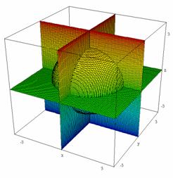
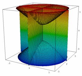
Spherical geometry: Fig. 1a: Geometry of a spherical surface in Euclidean space	Hyperbolic geometry: Fig. 1b: Geometry of a hyperbolic surface in Minkowski space

So the Euclidean geometry does posses a twin, the Minkowski geometry, which avoids curvature and hence satisfies the axiom of parallel lines. The two geometries share the affine structure of plane, i.e. they share:

Points Straight lines Parallel lines Ratios Midpoints Medians Translations Multiplications Similar figures
		Fig. 2

But is it also possible to give an elementary introduction to the Minkowski geometry avoiding abstract concepts such as the geometrical structure of space-time?

We suggest the following strategy: A Euclidean geometry is based upon a view on symmetry that makes the circle the most symmetrical figure – since ancient times considered the most perfect figure. This view e.g. dominated astronomy for several thousands years. But is it possible to imagine another view of the world, where it is not the circle, but the rectangular hyperbola, that is considered the most symmetrical figure? To make the transition to this alternative view more potent, we imagine that we follow Alice through the looking glass, and that she precisely discovers it is the alternative view, that prevails behind the looking glass:

4 Following Alice through the looking glass

Fig. 3: The most symmetrical figure as seen in front of the looking glass – behind the looking glass

The adoption of the rectangular hyperbola as the most symmetrical figure requires the introduction of new structures in Minkowski geometry:

Two asymptotic directions: Vertical/ horizontal

A different concept of right angles: We need to replace the traditional right angles, because of their intimate relationship with the geometry of the circle!

5 Right angles in the Minkowski geometry

To motivate the introduction of hyperbolic right angles we need some characteristic properties of a right angle, which links the right angle to a circle. Which property does not matter! We chose the following one, since this is a very basic one, easy to understand also on an intuitive level.

The tangent is perpendicular to the radius

To understand how tangents of a hyperbola behave we will use some analytical geometry. You may find this a little disturbing: Why not use elementary geometry all the way through. There are two reasons. The first one is that analytical geometry is in fact much simpler in relation to the Minkowski geometry than the Euclidean geometry. The second is that we lack intuition about the structure of figures in Minkowski geometry. For these reasons simple proofs in Minkowski geometry tends to be easier to follow using a little analytical geometry!

As a starting point we therefore take the following observation about the slope of a secant. By the way this is the only detailed argument based upon analytical geometry I will present in this paper. There will thus be lots of opportunities for the reader verifying results analytically later on your own!

The theorem of the secant

To determine the slope of a secant we perform the following standard calculation:

Fig. 4

Notice in particular that the slope of the secant only depends upon the product of the abscissa x! This has deep implications for the addition of hyperbolic angles!

To compute the slope of the tangent, we now simply let the two endpoints of the secant coincide. We thereby find the following well-known result:

Notice that we have managed to derive this elementary result without appealing to calculus! Next we compare the slope of the tangent to the slope of the radius:

Fig. 5

Conclusion: In Minkowski geometry two lines are perpendicular precisely when they have opposite slopes!

This observation is the main result. In particular it makes it easy to investigate simple properties of right angles!

6 Correspondences between the Euclidean and the Minkowski geometry

Recall the following theorems linking ordinary right angles to circles:

Example 1: First theorem of circles - Thales’ theorem: Fig. 6a: An angle is a right angle precisely when it spans the diameter

Example 2: Second theorem of circles - The theorem of Chords: Fig. 6b: The perpendicular bisector of a chord passes through the centre

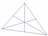
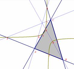
Example 3: Third theorem of circles - The circumscribed circle of a triangle:

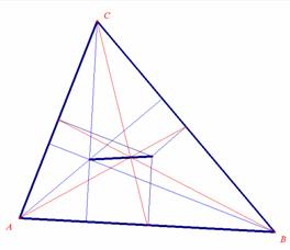
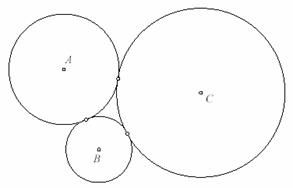
In each of the above cases it is elementary to verify the corresponding theorem in Minkowski geometry experimentally using a Dynamic Geometry program capable of drawing rectangular hyperbolas (a hyperbolic compass!). Fig. 7: The perpendicular bisectors of a triangle passes through the same point, the centre of the circumscribed circle

Other correspondences between the Euclidean and the Minkowski geometry involve the Euler line and the nine-point circle.

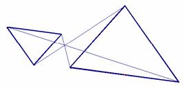
Fig. 8a: The Euler line in the Euclidean geometry	Fig. 8b: The Euler line in the Minkowski geometry
Fig. 9a: The nine-point circle	Fig. 9b:The nine-point hyperbola

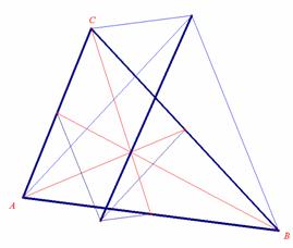
Notice that both cases are special cases of a theorem in affine geometry, which says that the heights in the triangle can be replaced by any set of three lines from the vertices passing through the same point. This gives rise to nine points through which a unique conic passes, the nine-point conic.

In the case of an ellipse, you may consider the configuration to be a parallel projection of the nine-point circle.

In the case of a hyperbola, you may similarly consider the configuration to be a parallel projection of the nine-point hyperbola.

In both cases the configuration is a shadow of a corresponding simpler configuration in Euclidean respectively Minkowski geometry. The above configuration with a nine-point conic is thus one of the places, where two separate theorems from Euclidean and Minkowski geometry are unified in affine geometry!

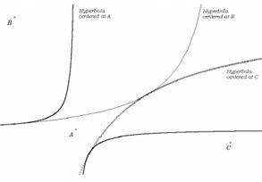
As a final example of such a correspondence we will look at the kissing circles. In Euclidean geometry any triple of points admits circles, which kiss each other (tangentially), in Minkowski geometry it is slightly more complicated, but in many cases you can still find kissing hyperbolas, see the following figure:

Fig. 10a: Kissing circle	Fig. 10b: Kissing hyperbola

Important remark: At this point you may perhaps think that all results in Euclidean geometries involving circles have a Minkowski counterpart. But that is not the case: The symmetry structure of the two geometries also has characteristic differences. E.g. rotations in Euclidean space have a repetitive periodic structure unlike the rotations in Minkowski space, where the asymptotic directions break the periodicity. As a consequence the Minkowski geometry lack regular polygons. And thus the regular polygons constitute an example of an important concept in Euclidean geometry, which has no correspondence in Minkowski geometry. But for pedagogical reasons we have emphasized the striking similarities rather than the (also important!) differences between the two twin geometries.

At this point you should now have obtained some feeling for the Minkowski geometry and we proceed with a discussion of the most basic theorem in Minkowski geometry – the analogue of the Pythagorean theorem, which controls all distance calculations!

7 Pythagorean dialogues between Alice and the Gryphon

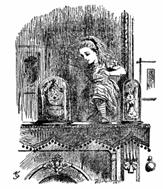
We present the derivation of the Pythagorean theorem in the form a dialogue between Alice, the Mock Turtle and the Gryphon starting with a famous dialogue written by Lewis Carroll for ‘Alice in Wonderland’:

'I couldn't afford to learn it,' said the Mock Turtle with a sigh. 'I only took the regular course.' 'What was that?' inquired Alice. 'Reeling and Writhing, of course, to begin with,' the Mock Turtle replied; 'and then the different branches of Arithmetic – Ambition, Distraction, Uglification, and Derision.' 'I never heard of "Uglification",' Alice ventured to say. 'What is it?' The Gryphon lifted up both its paws in surprise. 'Never heard of uglifying!’ it exclaimed. 'You know what to beautify is, I suppose?'

Fig. 11

A fictitious dialogue between Alice and the Gryphon about geometry:

‘I do suppose you know what a square is?’ the Gryphon exclaimed.

‘Of course’ Alice replied. ‘ It’s a totally symmetrical quadrilateral with four right angles’.

And to prove that she really understood what she was talking about, she made a sketch of a square:

Fig. 12a: Alice makes a drawing of a square	Fig. 12b:The Gryphon makes a drawing of a square

Alice claims the Gryphon’s square is a diamond, i.e. a rhombus with horizontal and vertical diagonals.

‘Oh no’, the Gryphon said in surprise: ‘That’s not a square – It’s just some silly parallelogram! This is how a square looks like!’

To Alice surprise the Gryphon made a sketch of a diamond figure. ‘Is that what a square looks like?’ she exclaimed.

‘Of course! Every child knows that a square has four right angles and is totally symmetrical! Don’t you learn anything in your schools? Didn’t they ever tell you about the Pythagorean theorem?’

‘Yes they did’, Alice replied cautiously, ‘ The Square of the hypotenuse is the sum of the Squares of the legs’.

‘What are you talking about’, the Gryphon replied, not believing what it just heard:

‘Every child knows that the square of the hypotenuse is the difference between the square of the legs’.

‘But I thought I had a proof?’ Alice dared to say.

‘Proof’, snorted the Gryphon. ‘You don’t even know what a square is!’

And the conversation continues with Alice demonstrating her proof and the Gryphon demonstrating his proof. Both use the same simple argument: First they decompose a square according to the formula for the square of a binomial:

(a+b)² = a² + b² + 2ab

Next they rearrange the figure suitably and the Pythagorean theorem follows immediately by comparing the two figures obtained in this way and ignoring the common right angled triangles:

Fig. 13a: Alice explains the Pythagorean theorem: c ^2 = a ^2 + b ^2

Fig. 13b: The Gryphon explains the theorem: b ^2 + a ^2 = 2b ^2 + c ^2 Þ c ^2 = a ^2 – b ^2

Remark: Once we have established the Pythagorean theorem for the Minkowski geometry we can make some important observations. There exist a Euclidean square, which is also a Minkowski square, namely the square with slopes ±1:

Fig. 14

It is then obvious to assign them this common square the same length of the side in the two geometries. Consequently the common square also gets the same area in the two geometries. Since collages of such special squares can approximate any simple figure, it follows that the area of any simple figure must in fact be the same in the two geometries. Thus they also have areas in common!

It is now easy to show that a rectangular hyperbola can be characterized as a set of points with constant hyperbolic distance to a center etc. Once we control distances we can also introduce trigonometry. In fact the socalled hyperbolic trigonometry is precisely the trigonometry associated with Minkowski geometry!

8 Angles in Minkowski geometry

As a preparation for trigonometry we must first introduce a measure for the hyperbolic angles (as opposed to the usual circular measure of angles). The starting point is a very important remark concerning addition of angles:

On addition of angles

Fig. 15a: Adding circular angles: P0Pu+v is parallel to PuPv	Fig. 15b: Adding hyperbolic angles: P0Pu+v is parallel to PuPv

The theorem of secants has the following important consequence:

The slope of P0Q:

The slope of PuPv:

Conclusion:

The hyperbolic angle is a logarithmic function of the associated abscissa since we get the following identity for the measure hyp(x) of the hyperbolic angle:

u + v = hyp(x₁) + hyp(x₂) = hyp(x₃) = hyp(x₁·^. x₂)

This makes it obvious to identify the measure of hyperbolic angle with the area of the sector OP0Pu, which makes sence, since on the one hand it is a well known fact – a fact that is elementary to verify! – that the area is also a logarithm function of the associated abscissa. On the other hand the circular angle is represented by an area in Euclidean geometry.

Comparison of angles in Euclidean and Minkowski geometry

Angles in Euclidean geometry (notice that the circle goes through the ‘unitpoint’ (1,1) and that the circle has the total area 2p, since the radius is Ö2!, see Fig. 16a).

Angles in Minkowski geometry: u = hyp(x) = Area(sector OP₀P_u).

Fig. 16a: Angles in Euclidean geometry	Fig. 16b: Angles in Minkowski geometry

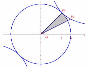
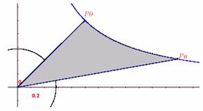
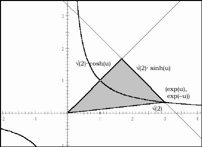
Conclusion: Hyperbolic angles generate natural logarithms: u = ln(x)

Notice that the hyperbolic measure of angles leads to a very simple canonical parametrization of the rectangular unit hyperbola, x y = 1, in terms of the anglular measure (hyperbolic ‘radians’). Since u = ln(x), we immediately get the abscissa expressed through an inverse natural logarithm, i.e. a natural exponential function: x = exp(u). The ordinate is the reciprocal value, i.e. y = exp(‑u). In contrast to ordinary trigonometry, where it is customary to introduce two trigonometric functions cosine and sine, we thus need only one basic trigonometric function for for the hyperbolic trigonometry: exp.

Canonical parametrizations in Euclidean and Minkowski geometry

a) The unit circle:	b) The unit hyperbola:
( x, y ) = ( cos(u), sin(u) )	( x, y ) = ( exp(u), exp(-u) )

9 Trigonometry in Minkowski geometry

This makes it possible to introduce hyperbolic trigonometry in precisely the same way you introduce circular trigonometry using right angled triangles:

Fig. 17

sin h (v) =

cos h (v) =

tan h (v) =

We leave the details as an exercise!

Goto
	Begin of article		Contributions by authors
	Begin of session		Main page

Cabri and anamorphosis

Chantal Gabriel-Randour and Jean Drabbe

Brussels, Belgium

Extended version in French

1. Introduction

2. Plane anamorphoses

3. Anamorphose of Piero della Francesca

4. Conical anamorphoses

5. Cylindrical anamorphoses

6. Pyramidal anamorphoses

1 Introduction

Anamorphic images are images, which have been distorted so that only by viewing them from some particular direction, or in some particular optical mirror surface do they become recognizable. There isn't much literature on the subject although some detailed descriptions were already published in the 17th century (e.g. "La Perspective Curieuse" by Père Jean- François Niceron - 1638). Most often, grid techniques or analytical methods are used. High school students, aged 17+ years from the Athénée Gatti de Gamond (Brussels - Belgium) were interested in anamorphoses. The students developed an approach mainly based on descriptive geometry. These constructions can easily be realized by using the Cabri-Geometry software. Different kinds of anamorphoses were treated in that way (plane, conical, cylindrical and pyramidal anamorphoses). The students' work was the subject of an exhibition held in Brussels in March 2001 involving also different aspects of the mirror in chemistry, physics, philosophy, history and geography. The following site shows a part of this work and references:

http://www.ibelgique.com/mathema

2 Plane anamorphoses

The linear perspective has been developed in Firenze at the beginning of XVth century by the architect, engineer, painter and sculptor Filippo Brunelleschi (1377-1446) and by Leon Battista Alberti (1404-1472). In 1436, Alberti achieved his work on the space representation Della Pittura. He is the first to state clearly the rules of the perspective.

Fig. 1	Fig. 2

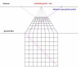
Here is the construction of Alberti when using Cabri. O is the vanishing point, the distance between O and D represents the distance between the eye and the picture, P is the point to represent and P’ is the point P in the picture.

3 Anamorphose of Piero della Francesca

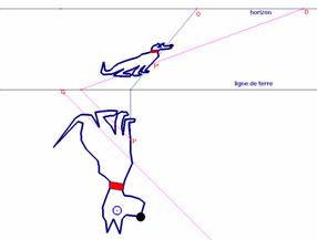
In de Prospectiva Pingendi, Piero della Francesca gave instructions for making a drawing so that the drawing seen from a given point gives the visual illusion of a bowl standing on a table. Fig. 3 the drawing made with Cabri following the instructions of Piero.
	Fig. 3

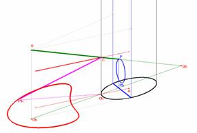
4 Conical anamorphoses

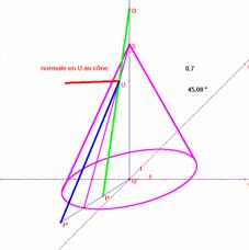
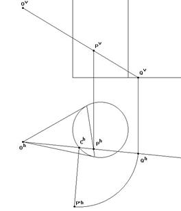
Imagine a right circular cone mirror standing on the ground plane and an eye point O directly above the tip of the cone. Just to make things easier, suppose that the vertical plane contains the eye point. Let imagine P a point in the ground plane. It is required to construct the point P' in the ground plane so that reflected in the mirror - seen from O - it appears to be P. In other words, P' satisfies the following condition.
	Fig. 4
Let OP intersect the cone at U. A ray from P' striking the cone at U is being reflected along UO. In case P is in the vertical plane, the problem is trivial. We are going to make use of this special case to solve the general problem. Rotate the ground plane around the (vertical) axis of the cone till P coincides with some point Q in the vertical plane and solve the problem for Q. This gives R. Apply the inverse rotation to R to find P'.
	Fig. 5

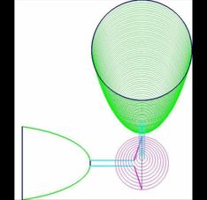
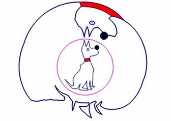
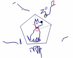
Fig. 6	Fig. 7: Conical anamorphose of a dog with Cabri - to be seen from infinity

5 Cylindrical anamorphoses

An eye point O and a cylindrical mirror standing on the horizontal (ground) plane are given. Let p be the plane of contact determined by the tangent planes to the cylinder from O. Let P be a point in p. It is required to construct the point P' in the ground plane so that reflected in the mirror - seen from O - in appears to be P. In other words, P' satisfies the following condition.
	Fig. 8
Let C be the point of intersection of the segment OP and the cylinder. A ray from P' striking the mirror at C is being reflected along PO. The key to the problem is the following remark. We let Q be the point of intersection of OP and the ground plane. The law of reflexion tells us that C^hQ^h = C^hP'^h .
	Fig. 9

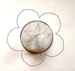
Fig. 10: Cylindrical anamorphose of a star using Cabri and its reflexion in the mirror cylinder

6 Pyramidal anamorphoses

Pyramidal anamorphoses may also been drawn with Cabri. The construction is developed on the site. Fig. 11 shows a pyramidal anamorphose of a dog when using Cabri.
	Fig. 11

Goto
	Begin of article		Contributions by authors
	Begin of session		Main page

Tabulæ and Mangaba:

Dynamical Geometry with a Distance Twist

Luiz Carlos Guimarães, Rafael Barbastefano and Elizabeth Belfort

Rio de Janeiro, Brazil

1. Introduction

2. Tabulæ

3. The communications mechanism of Tabulæ and Mangaba

4. Mangaba

5. Conclusions

We report on the ongoing development of two complementary DGS, for plane and space geometry. The design briefs of both computer programs were tailored bearing in mind the needs of distance teaching and Web communication. The current implementation is described in some detail, and we also discuss some of the issues that brought about the decision to engage in the project, as well as the implications for the technology driven teacher-training program that provided the initial motivation for it.

1 Introduction

In this paper we discuss a few of the distinguishing features of two DGS computer programs currently being developed by our group in the Laboratório de Matemática Aplicada of the Federal University of Rio de Janeiro.

From the outset we should make clear our reasons to engage in this development as, in our opinion, they might be of interest even for users of the well-established computer programs currently on the market. Of those reasons, by far the most determining for our decision was a consideration of cost and availability for the customers of our teaching projects: in service and prospective school teachers and, ultimately, the schoolchildren they are working with in state run schools. Cost alone puts this kind of computer programs out of the reach of nearly all teachers in Brazilian schools, let alone their students^[1].

On the other hand, the experience with this kind of computer programs at our University, where we could afford a site licence, provided other kinds of motivation for this project. Whereas the enthusiasm we observed in Rio for the laboratory classes is, we are sure, no news for anyone who has engaged in this sort of activities elsewhere, some needs have also emerged besides that of a platform affordable in a developing country like ours. We shall list below a few of them:

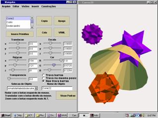
First of all, the lack of a convenient platform for space geometry. Although an experienced user might derive a lot of satisfaction from geometrical simulations in a 2dimentional platform, beginner students, who need most to develop their spatial skills, are not equipped to appreciate them. The current implementation of Mangaba (Fig. 1 below) goes some of the way towards addressing this need. In section 4 we describe some of its features.

A second consideration was that we wanted tools appropriate for distance teaching of geometry and for communication at a distance between students. Having developed the computer programs from scratch, it was possible for us to have built in facilities for communication. This approach contrasts with the (apparently easier) choice of adapting our computer programs to make use of a generic computer programs like Microsoft’s NetMeeting. There where sound reasons to go through the trouble of a specially designed communications server. We go into that in section 3.

Fig. 1: A scene on Mangaba

Last, and certainly not least, there was the issue of the freedom afforded by a home brewed platform, and the multiple benefits of engaging a taskforce of students learning diverse specialities in a truly multidisciplinary project. Through the bonding power of the common goal of completing computer programs directed at such a wide range of possible users, the project brings together students of engineering, computer science, mathematics, future teachers and students of product design. One major difference of our project as compared with other multidisciplinary groups elsewhere is the extensive involvement of undergraduate students.

2 Tabulæ ^[2]

Tabulæ is a dynamic plane geometry computer program, which has, at the moment we write, been a year in development. Entirely written in Java, in its current version it displays, as far as purely geometrical functionalities go, facilities similar to those available in Sketchpad and Cabri. What the current version still lacks, compared to them, is a proper scientific calculator interface, and a macro facility. As for this last facility, we are in the initial stages of designing a small programming language, which will, hopefully, allow the interfacing with a computer algebra language. The calculator is an easier matter, and is also in development.

On the positive side of the comparison, Tabulæ may already have a few points going for it:

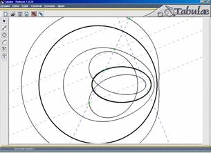
it allows the user to request that loci be drawn using an adaptive algorithm which is specially useful in degenerate situations, where the relevant construction points tend to cluster into a vanishingly small region of the parameter set. Compare, in Fig. 2 above, two equivalent situations drawn respectively with the latest available commercial version of Cabri (on the left), using its maximum 5000-point sampling, and with the current version of Tabulæ (with 200 point adaptive sampling). We understand the next version of Cabri will have a similar feature, and Cinderella Kortenkamp (1999) already uses an adaptive sampling algorithm. But in the case of Cinderella, the implementation adopted resorts to displaying only a few points of a locus while the mouse cursor is changing the parameters – a strategy no doubt made necessary by the overhead in processing speed of the Java program. We believe our solution will be more natural for the user;

Fig. 2: Nearly degenerate loci in Cabri and Tabulæ

Tabulæ’s graphical interface allows the user to choose, at any given step, between a “verb-noun” mode of construction and a “noun-verb” one (Bellemain 1992). A consultation to the files of the dynamical geometry discussion group at the Swarthmore Forum will reveal a spirited defence of each of the two modes, conducted by the designers of Sketchpad in one side and Cabri and Cinderella on the other^[3]. We feel that there are situations where either can have a definite advantage over the other, and leave the decision to the individual user,

Tabulæ’s design and execution are entirely object oriented, with the mathematical kernel and graphical interfaces completely separated in the program. The design allows easy additions and modifications in either component, and even the substitution of the mathematical routines with native code replacement,

Tabulæ allows a variety of different outputs. Besides it’s own file language, in XML format, the user can generate graphical files, in Postscript or GIF format, and a teacher can generate a report of commands and times from a student’s work session, a feature that can be useful for a maths education researcher,

Tabulæ can also output the Java code for a given session, much in the same way as Cinderella, which makes it an extremely useful tool for producing geometry hypertext materials. Allied with the VRML code generation of Mangaba, we feel that a teacher can have now at his/her disposal a unparalleled set of facilities for producing hypermedia with geometrical content,

and, of course, there is the communication capability, which Tabulæ shares with Mangaba. In the next section we give a succinct description of this facility.

Seemingly innocent design choices can have an extreme effect in the final capabilities of a mathematical computer programs. Fig. 3 below shows a construction where the circle and a ellipse (shown in thicker lines) are embedded into a one-parameter family of degree six algebraic curves. Constructions like those can provide very useful and motivating families of examples in a study of algebraic singularities (see Miranda 1995, Abhyankar 1990 and Griffiths 1989), but are not straightforward to obtain in Cinderella, due to its choice of implementation for the “point on object” primitive. As we have already mentioned in the introduction, one of the side benefits of writing the computer programs is that we can make sure it can be developed further to be useful for more advanced mathematical studies, as for instance in an algebraic geometry course.

Fig. 3: An one-parameter family of algebraic curves

3 The communications mechanism of Tabulæ and Mangaba

From the very beginning, mathematicians had to develop a special language of symbols, diagrams and text to communicate. The sophisticated interplay of these elements is already present even in the early texts of Euclid and Appolonius, as described in the thorough examination by Netz (1999).

As they started to use the WWW as a teaching and communication instrument, mathematicians were quick to realise the limits of working with a medium not initially designed for their trade, and to work to adapt it. Collective efforts like the Open Math Consortium (1998) and individual tours de force like D. Joyce’s (1997) transposition of the entire Euclid’s Elements into a set of Java powered HTML pages are two successful examples of that.

In this section we report on the development of a suite of computer programs designed to work together to provide an environment to teach mathematics, using the Web and specially designed computer programs for the student to work at home. One of the issues we address ourselves to is the fast generation and exchange of complex plane and three-dimensional geometrical constructions and simulations.

The goal of our application is to make possible the fast interchange of very complex objects, with a great degree of association. Think for instance of a tangent to a conic section, a geometrical locus, or of the large stellated dodecahedron.

The complexity of the objects to be shared by the users through a network dictated an unusual choice of implementation. Instead of the objects themselves, the communication server distributes only the behaviour of the users with respect to them. For instance, an object such as a dodecahedron, in a computer representation, has even more components than the original mathematical figure. Besides the original 20 vertices, the fact that each face has to be decomposed into triangles means that our dodecahedron is formed by 36 triangular faces. There are non-geometrical attributes to contend with as well, like colour and texture. In our approach this poses no problem, as the information to be transmitted through the network is mostly reduced to the object identifier (Id) and the construction identifier (CID). In other words, to transmit the instruction for the construction of a dodecahedron (or indeed the aforementioned stellated dodecahedron) is only marginally more complex than to transmit the instruction for a single point construction. Therefore the decision of distributing only the user’s behaviour through the network allows a significant step towards optimising the performance of the system.

Fig. 4: Reflection mechanism

4 Mangaba

In this section we report on the development of Mangaba, a tool for solid geometry. We briefly describe its main features, such as examples of building primitives, transformations and resources available for visualisation, object editing, import/export of code and the feature of construction sharing. We also discuss a few of the didactical possibilities that could be exploited through its usage in computers within elementary and secondary schools.

The study of solid geometry may well be the most efficient way available to us to develop in our students the kind of geometrical intuition, which, as argued by Penrose (1996), gives humans an edge over the calculating power of computers. Researches such as the one conducted by Tall (1991) suggest that a students' approach to more advanced mathematics is strongly influenced by his/hers previous set of experiences, and spatial visualisation plays an especially important role in this (Dreyfus, 1991a, 1991b).

Already at the beginning of the last century Poincaré (1952) pointed the distinction between geometrical space and representative space. According to his view, we sense and interact with objects in the representative space, but we reason as if they existed in geometrical space. Accordingly, the form we use to represent objects has an influence in our ability to understand their behaviour and properties. Therefore, modelling tools that may help students to overcome difficulties of geometrical visualisation in space can be especially useful, and it is no coincidence that the teachers taking part in our graduate courses display an keen interest in computational tools, which can model space geometry.

The subject has caught our interest and for a while now we have been researching both the possibilities of the languages JAVA and VRML (Guimarães et al, 2000) and of using two dimensional dynamical geometry computer programs to construct perspective representations of spatial figures (Gani and Belfort, 2000). This experiments are still being continued, but the limitations in both approaches are already very clear.

Whereas a VRML microworld privileges spatial visualisation, allowing unrestricted movement of the whole scene and even a limited degree of programmed-in relative movement, there are no provisions for constructions to be effected by the user, and his/her role is limited to manipulating previously prepared scenes.

In a (plane) DG environment, on the other hand, an user can use the language of descriptive geometry to construct his/her own objects, but the visualisation possibilities are severely impaired by the medium. Perspective representation and a language of stylised graphical conventions (such as differentiated line thickness, traced lines to represent hidden edges, etc.) have to be used to foster the impression of three-dimensionality. Even though a mathematically correct construction may yield a figure with some movement, it is in general not possible to build into the conventional graphism a coherence with all possible positions of the figure. Nevertheless, our experience bears witness to the fact that, on the hands of a capable teacher, DG figures coupled with descriptive geometry can play a very important role in the classroom.

On the basis of the experiments and difficulties reported above, it became clear to us that a computational tool which allowed the user to build his/hers own figures while seeing them in an environment similar to that provided by a VRML viewer was worth the investment.

Mangaba is designed to be a space geometry counterpart of Tabulæ, retaining the same facilities as a tool for communication through the Internet and the variety of specialised outputs available to the user. Compared to Tabulæ, the present version is still in a very early stage of development, but the features available at this stage already make it a fairly complete three-dimensional editor.

Given the amount of work involved in the geometrical construction of complex objects in space, we were led to work with a much larger set of primitives than those needed in Tabulæ. This is also necessary in order to keep the size of objects down to the minimum necessary.

General-purpose CAS computer programs like Maple can generate spatial objects but, in our experience, the artefacts so generated tend to be too large for our purposes (Guimarães et al., 2000). The set of primitives already available in Mangaba includes an extensive set of polyhedra (convex or otherwise) as well as the usual figures and solids to be found in textbooks in Euclidean space geometry. Given two primitives, a third can be specified as a special join of the two given objects, so that for instance a two leafed cone can be generated from two copies of a one leaf one.

The primitives can be edited and geometrically transformed in a number of ways, including the usual affine transformations (more complex non-linear transformations are still in the drawing board). Non-geometrical attributes like colour, transparency, textures and lighting are available for editing figures as well.

A set of geometrical construction tools is being developed, with a skeleton sample already available. A step due next, starting this quarter, is the integration in this computer programs of the tools available in Tabulæ. The idea is that, inside a Mangaba microworld, once the user selects a given plane in space, the full set of construction tools of Tabulæ would be made available for use in that plane. This, together with the purely spatial construction tools already available (like plane/plane and plane/sphere intersections) will, we believe, go a long way towards establishing Mangaba as a true solid DGS.

5 Conclusions

The use of computer programs as an auxiliary support for the student in distance courses of Mathematics is becoming more and more common, the Open University in Great Britain being an important case in point. In the case of the OU undergraduate degree courses, the decision to use a general purpose CAS (MathCad) seems to be a sound one, given both the potential usefulness of the tool in their students future careers and the ready availability of grants for their students. Unfortunately, the same conditions do not necessarily apply in the case of a school Mathematics teacher in other countries.

Recent research reports and panel recommendations in several countries point out the importance of teacher training as a prime factor in the quest for better results in the school system (see for example Kilpatrick et al, 2001). There seems to be a great deal of room for experiments on the use of distance education technology in training programs directed at improving the mathematical knowledge of the teaching workforce.

Take for instance the Brazilian school system as a case in point, with its nearly 50 million students currently in elementary and secondary schools. There is no way the existing network of Mathematics departments in Brazilian universities can possibly cope with the task of giving initial and in service training for the huge numbers of teachers needed for the discipline, unless we can resort to efficient distance teaching networks.

It would seem that very specific tools would be needed if we want to develop this kind of distance teaching networks, particularly those that can help to develop geometrical visualisation and reasoning. In our case, the first samples of teaching materials designed for use with Tabulæ and Mangaba are under development. The results of the first pilot tests are encouraging. More on that, and on MatChat, a tool to integrate a CAS into an environment designed for synchronous distance teaching through the Internet, can be found in (Guimarães et al, 2002).

Acknowledgements. Research partially supported by CNPq. We thank the team who is making these computer programs possible: Alexandre Tessarollo, Aline S. Ferreira, Bruno Rothgiesser, Celso G. Barreto Júnior, Diego Carvalho, Fábio G. Menezes, João Carlos S. Freitas, Leonardo F. Almeida, Rodrigo S. Moreira, Rodrigo A. Hausen, and Thiago G. Moraes.

References

Abhyankar, S. (1990) Algebraic Geometry for Scientists and Engineers. AMS.

Bellemain F. (1992) Conception, réalisation et utilisation d'un logiciel d'aide à l'enseignement de la géométrie: Cabri-géomètre. Ph.D. Thesis, Universidade Joseph Fourier, Grenoble.

Dreyfus, T. (1991a) Advanced Mathematical Thinking Processes. D. O. Tall (ed.) Advanced Mathematical Thinking. Kluwer, London.

Dreyfus, T. (1991b) On The Status of Visualisation and Visual Reasoning. Mathematics and Mathematics Education. Proc. 15th Psychology of Mathematics Education Congress, vol 1, 33-48. PME, Assisi.

Gani, D. C. & Belfort, E. (2000) Descritiva em Geometria Dinâmica: Integrando Representações. Annals of GRAPHICA 2000, (electronic edition). UFOP, Ouro Preto, MG.

Griffiths, P. (1989) Introduction to Algebraic Curves. AMS.

Guimarães, L. C.; Barbastefano, R and Belfort, E. (2000) Tools for Teaching Mathematics: A case for Java and VRML. J. of Comp. Applic. in Engin. Educ. 8, n. 3-4, 157 -161.

Guimarães, L. C.; Barbastefano, R and Belfort, E. (2002) Tools for Synchronous Distance Teaching in Geometry. Proc. the 2nd Intern. Conf. on the Teach. of Math. (ICTM2), to appear.

Hartshorne, R. (2000) Geometry: Euclid and Beyond. Springer.

Jackiw, N. (1997) The Geometer’s Sketchpad. Key Curriculum Press.

Joyce, D. (1997) Euclid’s Elements. http://aleph0.clarku.edu/~djoyce/java/elements/ elements.html

Kilpatrick, .J, Swafford, J. and Findell, B. (ed.) (2001) Adding it up: Helping Children Learn Mathematics. National Academic Press, Washington, DC.

Kortenkamp, U. (1999) The Dynamical Geometry Computer programs Cinderella. PhD. Thesis, ETH, Zürich.

Miranda, R. (1995) Algebraic Curves and Riemann Surfaces. AMS.

Netz, Reviel (1999) The Shaping of Deduction in Greek Mathematics: A Study in Cognitive History. Cambridge U. P, Cambridge.

Penrose, R. (1996) Mathematical Intelligence. Khalfa, J. (ed.) What is Intelligence? Cambridge U. P, Cambridge.

Poincaré, H. (1952) Science and Hypothesis. Dover

Tall, D. O. (1991) Reflections. D. O. Tall (ed.) Advanced Mathematical Thinking. Kluwer, London.

The OpenMath Consortium: www.openmath.org

Goto
	Begin of article		Contributions by authors
	Begin of session		Main page

Computer experiments

in the lecture of analytical geometry

Victor Lysytsya

Kharkov, Ukraine

Analytical geometry is one of the parts of higher mathematics, which is taught at the faculties of Physics and Mathematics and practically at all faculties of Technical Higher educational establishments. Elements of Analytical Geometry are also taught at school as part of the curriculum. It is known that analytical geometry studies characteristics of geometric figures by analytical methods.

This method is founded on the method of coordinates, which has been used first and systematically by René Descartes (French mathematician and philosopher, 1596-1650). The method of coordinates is a very deep and powerful device, which allows using the methods of algebra and mathematical analysis for studying of geometric objects. Besides this method is characterized by visual graphic demonstration that gives the possibility to use pictures within the context when you teach the majority of chapters of analytical geometry.

When you study the geometric objects one should observe the dynamics of characteristics of the figures when the corresponding parameters have been changed. When you use classic methods such observation is next to impossible, especially when parameters are being changed constantly in any sphere.

Classic ways of studying geometric objects that is use of such tools as compasses and ruler can be glanced at from a new point of view with the appearance of computer technologies. These tools are realized in the well-known packets: Cabri, Sketchpad.

It should be mentioned that methods of task solution are changed when computer methods of research are used. So, the application of special geometric packets during studying geometric figures is worth trying.

Some tasks in the lecture “Analytical geometry” where one can use the possibilities of experimental research with the help of DG packet are suggested here. This DG packet has been suggested by the group of mathematicians and programmers (the scientific advisor is assistant professor S.A. Rakov, Kharkov State Pedagogical University after G. Skovoroda).

One of the most important chapters of analytical geometry is the chapter where coordinates on the plane have been introduced.

Characteristics of geometric figures are proved with the help of coordinate method, equations are received, and the form is studied. It should be noted that analytically “ compasses and ruler” – these are circle and straight line.

Tasks directed at the research of geometrical sets of points without use of analytical formulas but with the use of classic tools are suggested in this paper. Let us give examples of some tasks from this chapter. First of all let’s remember that in the topic where Cartesian coordinates are analysed the formulas of distance between two points are given, formulas for the coordinates of the point, which divides the segment in the given parts.

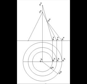
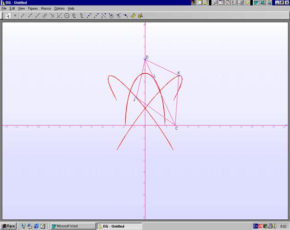
Task 1.

Triangle CDK by its apexes C and D slips along orthogonal coordinate axis. Analyse the curves, which the third apex K draws and point L on the side CD, which divides this side in the proportion CL:LD = l. How will the curve be changed when parameter is changed?

With the help of the packet DG one can make an experiment and draw curves, which the points A and M make (Fig. 1).

Let us notice that the points J and K are symmetric to CD. It can be easily seen that the curves, which they draw, are symmetric to the axis OY. The analysis shows that these curves are ellipses.

Fig. 1

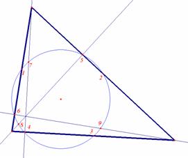
Task 2: Circle of Apollonium

Find a set of points of the plane, proportion of distances of which to the points A and B is constant and is equal to k. Picture 2 shows the results of the experiment made.

Fig. 2

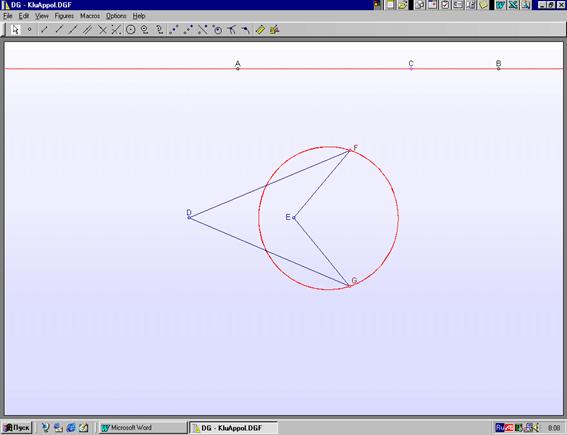
Distance between two points A and B is changing, but AC : CB =k. The experiment is made in such a way that DF =DG =AC, EF=EG=BC.

References

Pogorelov, A.V. (1983) Geometry.Science. Moscow.

Ilyin, V.A., Poznyak, E.G. (1971) Analytical Geometry. Science, Moscow.

Rakov, S.A., Goroh, V.P. (1996) Computer experiments in geometry. Kharkov.

Goto
	Begin of article		Contributions by authors
	Begin of session		Main page

Fig.: Hochosterwitz castle in Carinthia

Learning explorations and its DG support

in the geometry course for secondary schools

Valentyna Pikalova

Kharkov, Ukraine

Deductive reasoning lies at the core of any cognitive process. This ability can be successfully developed during problem solving tasks in geometry course of secondary school. Great pedagogical potential can be found in computer based geometry syllabus as Dynamic geometry enables a learner not only visualize geometric transformation but also motivates active search for an effective variant of solving this or that problem.

In the course of our research geometric changes proved to be a powerful tool in developing insight into obtaining the correct solution. The ability to discard the false hypotheses can be effectively formed by dynamic geometric transformations. DG tasks also create highly stimulating exploration environment.

And now we would like to share with you some of our observations based on 2-year pedagogical experiment in Kharkov State Pedagogical University, the objective of which was to find out how DG tasks stimulate cognitive process of spatial visualization and in what way they facilitate the learning process. The group of 12 students was taught the DG syllabus. The check group included 6 students from the same university. The students were offered to choose the topic from the geometry course for secondary school (triangles, Pythagorean theorem, quadrilaterals, polygons, geometric transformations, vectors) for their independent analysis in the terms of adaptability of tasks to the methods of dynamic geometry. Further on they had to devise their own tasks and test them in classroom situations. And next year the group of 10 students made a practical use of their deductive material. They also tested DG software devised at the department of computer science of the university.

Our observation can be summed as follows:

Students can generate many examples as a way of forming and exploring conjectures, but it is important for them to recognize that producing many examples of a particular phenomenon does not constitute a proof.

Constructing geometric objects in dynamic geometry environment puts a leaner into the framework of an algorithm conception. Macros recoding plays an important role in analysing geometric relationships.

An accurate drawing is of paramount importance as it helps exclude a lot of potential mistakes during tasks solving.

Some geometric models cannot be constructed with the help of classic tools (compasses and ruler), for example the angle trisection, so DG tools can be successfully applied. A vivid support to this argument can be gained by considering classical Morley theorem: three trisectors are constructed in each angle of the triangle ABC. Build three intersection points of adjacent trisectors. Investigate the triangle with vertices in intersection points (the trisectors of an angle is a two lines or rays that divides an angle into three congruent adjacent angles). As you see in Fig.1 we have the right triangle with vertices in intersection points of adjacent trisectors. The drawing in this case gives an important clue to this solution and helps formulate a hypothesis. Use the macros to construct trisectors (for building macros you need the analytic point tool).

Fig. 1

Another positive factor of DG tasks can be formulated as such: Dynamic geometry software is an optimal tool for analysing characteristics and properties of geometric shapes and developing mathematical arguments about geometric relationships. For example, we can apply measurement tools to explore properties of special quadrilaterals (parallelogram, rhomb, rectangle, square etc.).

Dynamic geometry enables a learner to apply transformations as a tool for problem solving and analysing a mathematical situation.

Computer based experiments stimulate cognitive search of possible solving. The students’ valuable research experience is formed, which enables learners to turn into active explorers instead of remaining passive observers. The process of storing different strategies is the part of the growth of learners’ geometrical expertise.

The process of teaching and learning diverse approaches of one problem solving plays an important role in mathematical reasoning. Sometimes it is preferable to solve one task in different ways rather than many different tasks in one way. Applying miscellaneous methods for task solving helps find out advantages and disadvantages of a particular method and see how logically justified this method is. We would like to give some examples of DG tasks designed in the form of learning explorations for solving the given problem in many ways.

Problem. Construct midpoints K, L, M and N on each side of the quadrilateral ABCD respectively. Join consecutive points to get the quadrilateral KLMN. Conjecture the ratio between values of areas of quadrilaterals KLMN and ABCD (Fig. 2). Test your conjecture by dragging vertices A, B, C, D.

Consideration. Construct the model and then measure the areas of quadrilaterals KLMN and ABCD. Measure the ratio ABCD/KLMN. Change the position of any vertex of the quadrilateral ABCD. Conjecture about the ratio ABCD/KLMN.

Let us prove the hypothesis using different strategies.

Strategy 1. Pay attention to the triangle ACD and the segment NM (remember, that N and M are midpoints of sides AD and CD respectively).

Fig. 2

Draw the parallel line to the diagonal AC through the point N. Conjecture about the relationship between the segment NM and the diagonal AC.

As you know the segment whose endpoints are the midpoints of two sides of a triangle: a) is parallel to the third side; b) its length is half the length of the third side. Therefore NM=AC/2.

Take the point S₁ on the segment AC. Draw the segment DS₁ and its intersection point E₁ with the segment MN. Measure segments DE₁ and E₁S. Conjecture about the ratio DE₁/E₁S. Test your conjecture by dragging the point E₁.

Draw the perpendicular from the point D to the opposite side. The segment MN divides the perpendicular DS into two equivalent parts: DE = ES (Fig. 3). You can use for proving the theorem: if three parallel lines cut congruent segments off a transversal then, they cut off congruent segments on every transversal.

Fig. 3

The area of a triangle is the product of half the length of its base and the length of the height, therefore S_ADC = ½ DS·AC; S_NDM = ½ DE·MN = ½ DS/2·AC/2 = ¼ S_ADC.

Conjecture about the area of the triangle LBK. Investigate the value S_NDM + S_LBK.

Apply the same strategy to triangles ANK and CML.

Use S_ABCD = S_ADC + S_ABC = S_CBD + S_ABD to finish proving.

Strategy 2. Construct the model: Draw parallel lines to diagonals AC and BD through vertices of the quadrilateral ABCD. Construct the quadrilateral A₁B₁C₁D₁ with vertices in points of intersection of constructed parallel lines (Fig. 4).

Investigate the relationship between areas of triangles ADD₁ and ADO. Conjecture about the relationship between areas of quadrilaterals ABCD and A₁B₁C₁D₁.

Investigate the relationship between areas of quadrilaterals AD₁DO and FNEO. Conjecture about the relationship between areas of quadrilaterals KLMN and A₁B₁C₁D₁.

Use the ratio S_A1B1C1D1/S_ABCD and the ratio S_A1B1C1D1/S_KLMN to finish proving.

Fig. 4

Strategy 3. The point O of the intersection of diagonals AC and BD joined by segments with vertices of the quadrilateral KLMN. Explore 4 pairs of triangles: AKN and OKN, BKL and OKL, CLM and OLM, DMN and OMN.

The final stage of the experiment was scientific research collaboration with students. The theoretical and practical results were accounted for by the students at the seminar supervised by Prof. Sergey Rakov. The seminar revealed such psychological changes in learners’ cognitive approaches:

The students get an immediate grasp of the research content of the problem rather than when given an ordinary academic task.

DG enhances their exploration instincts so that they can discover some adjoining problems while solving the task.

Having been exposed to a new stimulating research-oriented and thought provoking teaching the students sounded very optimistic about using DG tools in their future work of math teachers.

Computer based plane geometry course for secondary school and Dynamic Demonstrative library (which consists of dynamic sketches for learning explorations) came out as a practical application of the experimental work which is due to be implemented in Kharkov secondary schools in 09/2001 – 05/2002.

References

Rakov, S.A., Gorokh, V.P. (1996) Computer Experiments in Geometry (in Russian). RCNIT, Kharkov.

Rakov, S.A., Pikalova, V.V. (2000) Computer Practice for Students from Pedagogical University as Preparation for Using Mathematics Packages in Secondary School Curriculum (in Russian). Information Technologies: Science, Technologies, Education, and Health. Collection of papers. Kharkov, 198-202.

Goto
	Begin of article		Contributions by authors
	Begin of session		Main page

Voronoi diagrams produced by DGS

as a tool in an educational study

Harry Silfverberg

Tampere, Finland

1. Classification of geometric figures

2. An attempt to study the prototypical classification of triangles

The Voronoi diagram of a collection of points is a partition of space into cells, each of which consists of the points closer to one particular point than to any others. According to the prototype theoretical explanation, students at the lowest van Hiele levels tend to classify geometrical figures on the basis of extent of the similarity of the figure and the visual prototypes. In this paper I will discuss about the possibilities of using Voronoi diagrams as a tool in studying the ways in which students at the lowest van Hiele levels classify a given collection of triangles into acute, right, obtuse, equilateral and isosceles triangles. In my presentation I will further show how the Voronoi diagrams and partitions based on the different selection of prototypes fit to the empirical data gathered in Silfverberg (1999).

1 Classification of geometric figures

According to the Platonic view, geometric concepts are ideal objects, which get their conceptual meaning through mathematical defining. Classical abstraction theoretical explanation has been that the learning of the well-defined concepts proceeds through the steps shown in Fig. 1.

Fig. 1: Abstraction theoretical (classical) explanation of the learning process of geometric concepts

Although the basic geometric concepts of the school geometry are in principle easily definable and the definitions of the concepts are presented in almost every textbook, students conceptual understanding don't normally base on the definitions. Many students seem to understand geometric concepts analogously as they understand natural concepts like a table, a dog etc. They know the typical instances of the concepts but they can't formulate exact definitions to the concepts. From the point of view of van Hiele theory it means that these students' geometric thinking show the typical features of the two lowest van Hiele levels.

On the first van Hiele level (vH1) the focus of student's geometrical thinking is on the visual image of the figure.

On the second van Hiele level (vH2) the focus of the geometrical thinking gradually shifts to the properties of the figures.

An ability to define concepts and an ability to apply the definitions in geometrical reasoning is normally not reached before the level vH3. On that level the focus of student's geometrical thinking shifts to the relations of the properties, which makes it possible to a learner to express the meaning contents of the concepts exactly. However, many students have difficulties in using definitions as a basis of their reasoning also on the level vH3. For instance in Silfverberg's (1999) research most of the students, who were classified to that level, didn't clearly understand what the defining process actually means.

Because students, who are on the van Hiele levels vH1 and vH2, can't use definitions as a tool in classification tasks they have to base their decisions more on the so called prototypical classification, which is done on the basis of comparing the overall similarity of the example figures and the visual prototypes of different categories. The prototypical classification normally leads to fuzzy boundaries of categories. As a process it is very different from the classification, which is based on the knowledge of the definitions of the concepts. In the prototype theories it has been suggested different explanations to the origin of the prototypes.

For example according to the feature averaging model (fam), typical members contain the mean or average values of attributes that are varying within the category whenever these attributes vary on metric for which an average can be "calculated". According to the feature frequency model (ffm), typical members contain the most commonly experienced values of attributes that are varying within the category when these values can be "counted" (Strauss 1979).

Although students, who are on the van Hiele levels vH1 and vH2, normally lack for example the ability to correctly classify all the given example triangles into acute, right, obtuse, equilateral and isosceles triangles, they however, can quite correctly classify the typical examples of the different types of triangles. The less typical the example figure is the smaller is also the probability, that the classification of the given example goes right.

Fig. 2 shows how the prototypical concept formation precedes the more abstract concept formation and how it leads to two different classification procedures.

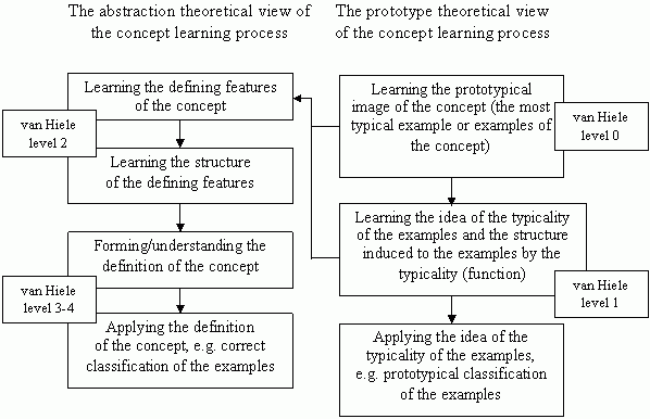Fig. 2: The combination of the prototype theoretical and the abstraction theoretical explanations of the learning process of the categorisation of the geometric concepts

2 An attempt to study the prototypical classification of triangles

The method

In the following I will sketch one possibility to model the phenomenon of prototypical classification attached to the classification of different types of triangle concepts. The main steps in that modelling process will be (1) the representation of different classes of triangles on a two dimensional co-ordinate system, (2) the selection of hypothetical prototypes to different types of triangles, (3) the construction of the dynamical Voronoi diagrams induced by the prototypes, (4) the selection of probability function, which expresses the typicality of the example compared to the prototype, and (5) evaluation, how well the constructed model(s) will fit to the empirical data of classification of triangles.

Coding the shapes of the triangles to the points of the two dimensional conceptual space

As a fact there are several ways to represent every possible shape of a triangle as a point in plane. Such representation forms then a model, which Gärdenfors (2000) calls, as a conceptual space. One possibility to do that is to code the shape of each triangle by the ordered pair of numbers (x, y), where x Î [60^o,180^o[ is the biggest and y Î ]0^o,90^o[ the second biggest angle of the triangle.

From the definition of x and y it follows that y £ x, x + y < 180^o and y > 180^o - (x+y) e. g. x + 2y > 180^o. The points (x, y), which fill these restrictions, locate in a triangle ABC, where A is (60^o,60^o), B is (180^o,0^o) and C is (90^o,90^o), excluding the side BC. So each triangle (shape) can be represented by an inner point of the triangle ABC or by a point on the half open segments AB or AC.

Fig. 3: Representation of shapes of triangles by points in plane

DynamicVoronoi diagrams induced by the prototypes of the different types of triangles

The Voronoi diagram induced by the a set of points {P₁, P₂, ..., P_n} in plane is a partition of the plane into cells such that for each cell corresponding to the point P_i , i = 1, ... , n the points P in that cell are nearer to the point P_i than to any other point of {P₁, P₂, ..., P_n}. The sides of the Voronoi cells are segments, rays or straight lines going along some of the perpendicular bisectors of the segments P_iP_j, i=1, ... ,n, j=1, ... , n, i¹j.

Fig. 4: Voronoi diagram induced by the set {P1, P2, P3, P4}

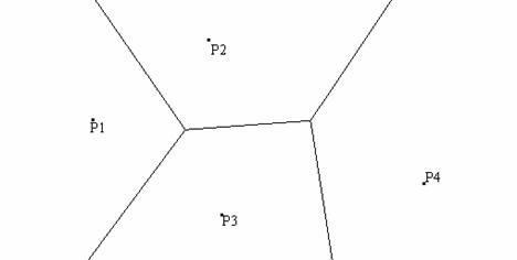
Fig. 4 is made by the Cabri application downloaded from http://140.114.32.3/chuan/cabri-work/figures/Surprises/. There are many sites in web

http://wwwpi6.fernuni-hagen.de/Geometrie-Labor/VoroGlide/, http://www.msi.umn.edu/~schaudt/voronoi/voronoi.html, or

http://www.cs.cornell.edu/Info/ People/chew/Delaunay.html,

where it is possible to construct dynamical Voronoi diagrams, which change dynamically as the user changes the number of the points P₁, P₂, ..., P_n generating the diagram or the location of these points. With the help of DGS it is also possible to construct dynamical Voronoi diagrams locally.

Properties of the typicality function

Let C(P_i) denote the cell of the Voronoi diagram generated by the prototype P_i and d_i the Euclidean distance from the point P Î C(P_i). It is often assumed that the similarity s_i of the example P and the prototype P_i is a function of the distance d_i between the P and P_i in the underlying conceptual space. Many researchers have proposed that similarity is an exponentially decaying function of distance (cf. Gärdenfors 2000, 20). However, it is evident that also all the neighbouring prototypes affect somehow to the classification process and if we want to determine the probability that the example corresponding to the point P Î C(P_i) will be classified to the category determined by the prototype P_i we have to take account other competing prototypes. Let us simplify the task and restrict our discussion to two prototypes P_i and P_j.

Fig. 5: Euclidean distances di and dj from point P to the prototypes Pi and Pj

Let p_ii be the probability that the example corresponding to the point P Î C(P_i) will be classified to the category, which prototype is P_i, and p_ij the probability that the same example will be classified to the category, which prototype is Pj. Our task is to find a typicality function of di and dj which give the right empirically verified classification probabilities p_ii and p_ij so that, if P = P_i , then p_ii = 1 and p_ij = 0 and, if P lies on the boundaries of the neighbouring cells C(P_i) and C(P_j), then p_ii = p_ij.

Constructing and testing the model

With dynamic geometry software like GSP or Cabri Geomètre it is possible to construct a model of the prototypical classification process of triangles, where

triangles are coded and represented as points in a plane as in Fig. 1,

the hypothetical prototypes for each category are selected,

the Voronoi diagrams generated by the prototypes are constructed and

theoretical probabilities to different types of classifications are calculated.

The dynamical model of classification process can then be evaluated by checking how well the model can predict the results, which have got in classification tests where different example triangles have been classified to different types of triangles (for example results in Silfverberg's study 1999). The dynamics of the model makes it possible to find the best fitting results either changing the selection of the prototypes or the selection of the probability function or both. The selection of the prototypes is dependent for example to the position, which is taken to the origin of the prototypes (see fam and ffm above). Some suggestions for the possible choices for prototypes and typicality functions will be given in an oral presentation in the conference.

References

Gärdenfors, P. (2000) Conceptual Spaces. The Geometry of Thought. MIT Press, Cambridge, Massachusetts.

Silfverberg, H. (1999) Peruskoulun oppilaan geometrinen käsitetieto. [The conceptual geometric knowledge of pupils in the upper level of comprehensive school] Ph.D. thesis. Acta Universitatis Tamperensis; 710, 254 s. Tampereen yliopisto, Vammala.

Strauss, M.S. (1979) Abstraction of Prototypical Information by Adults and 10-Month-Old Infants. Journal of Experimental Psychology: Human learning and Memory 5 (6), 618-632.

Goto
	Begin of article		Contributions by authors
	Begin of session		Main page

Use of Cinderella in higher elementary geometry

Hermann Vogel

München, Germany

Interactive version of the paper

1. Illustration of well known facts using move and animation modes

2. Discovering of new conjectures doing interactive exercises

3. Creating the envelope of a set of straight lines

4. Construction of conics determined by certain conditions

5. Creation of algebraic curves of higher order

This paper shows the possibilities of presenting advanced Euclidean geometry on an HTML-page with the interactive geometry software Cinderella. It deals with the well-known Wallace-line and a generalization of this line invented by Giering (1998). More details about an in-service training course for teachers may be found at

http://www-m1.ma.tum.de/lehrer/material/elementargeometrie .

1 Illustration of well known facts using move and animation modes

We consider the pedal triangle PQR of the triangle ABC with respect to the point X. We ask for the locus of X while the pedal triangle degenerates into a line of collinear points [PQR]. This straight line is called the "Wallace-line of the triangle ABC with respect to the point X". This line is also called Simson-line. Using the move mode in Fig. 1a we see, that the solution is the circumcircle u of the triangle ABC. This is an example for the useful tool "Bind a Point on a Line", which will be available in version 2 of Cinderella. Fig. 1b shows the solution.

Fig. 1a

Fig. 1b

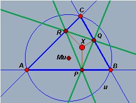
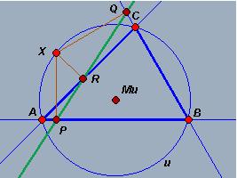
2 Discovering of new conjectures doing interactive exercises

Fig. 2

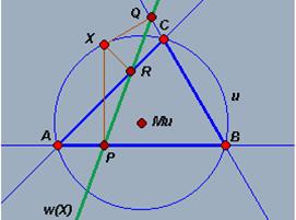
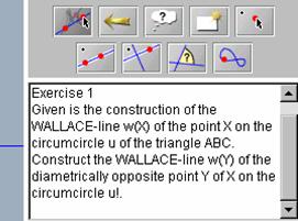
We are led through this exercise 1 in Fig. 2 by clicking the "Questionmark Button" in the toolbar. Doing this we get additional hints as well as new questions and answers prepared by the teacher in the exercise console. Alternatively, we can use the tool buttons and go through the exercise by ourselves. We will get some information, comments and new questions in the exercise console as well. The result of this exercise is the following: The two Wallace-lines of diametrically opposite points X and Y on the circumcircle of a triangle are perpendicular and the intersection point of these lines lies on the nine-point circle. For the nine-point-circle the teacher could prepare a hyperlink to more details.

3 Creating the envelope of a set of straight lines

Now we look for the envelope of the Wallace-lines of a triangle ABC. With Cinderella we create this envelope using the locus mode by selecting the point X as the mover, the circumcircle u as the road and the Wallace-line of X as the tracer. The result is the hypocycloid of Steiner with three cuspidal points and the circumcentre N of the nine-point circle as the centre of a three axes symmetry. There is an interesting relationship with the Morley-triangle of the triangle ABC too. Fig. 3 shows this hypocycloid as the envelope of the Wallace-lines using the animation mode; Fig. 4 shows an alternative creation of it as a roulette.

Fig. 3

Fig. 4

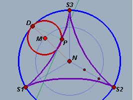
We get more nice figures, if we look for a first generalization of the Wallace lines. Let X be a point on the circumcircle u of a triangle ABC. Instead of perpendicular lines we consider the isoclinal lines through X rotated by the angle a and get a straight line [P*Q*R*] as well.

Fig. 5a

Fig. 5b

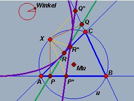
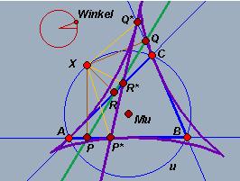
Fig. 5a shows the envelope of the lines [P*Q*R*] changing a and leaving X fixed. We get a parabola with the focus X and the Wallace line [PQR] as the tangent at the vertex. Fig. 5b shows the envelope of the lines [P*Q*R*] leaving a fixed and moving X. We get a hypocycloid of Steiner again.

4 Construction of conics determined by certain conditions

For a second generalization of the Wallace-lines we look for the other intersection points of the perpendicular lines to the sides of the triangle ABC through a point X with the sides of the triangle ABC called P', Q', R' and P'', Q'', R''. Now we ask for the locus of X while the points P', Q', R' or the points P'', Q'', R'' are collinear.

By algebraic considerations we find out, that this locus consists of two conics. One for the collinearity of [P'Q'R'] called the Wallace-right-conic c' and the other one for the collinearity of [P''Q''R''] called the Wallace-left-conic c''. With Cinderella we can create each one, if we have five points, which lie on the conic. In the interactive exercise 2, Fig. 6, we look for such points on the Wallace-right-conic c':

Fig. 6

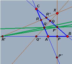
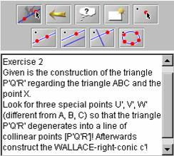
First we move the point X to get an idea of the solution. After a while we can see that the intersection point of the perpendicular lines of the line AB through the point B and the line BC through the point A is one of these points. By cyclic permutation we get three special points. Of course, the points A, B, C lie on the conic, too. Alternatively, we can do this exercise as well by clicking the "Questionmark Button" in the toolbar.

With the result of this exercise we get two congruent conics c' and c'' with perpendicular axes, see Fig. 7. These conics belong to the set of the circumscribed conics of the triangle ABC, which has the four centres A, B, C, D on the circumcircle u. So we have discovered a new remarkable point D of the triangle ABC.

By creating the point D as an intersection point of the two conics Cinderella reports in an information console that D lies on the circumcircle u of the triangle ABC. So Cinderella gives us a strong evidence, that our conjecture is true by a technique called "Randomized Theorem Checking". Unfortunately this information console doesn't exist for HTML-pages.

In Fig. 7 one can discover more interesting facts, but here is no space to explain all of them.

Fig. 7

Fig. 8

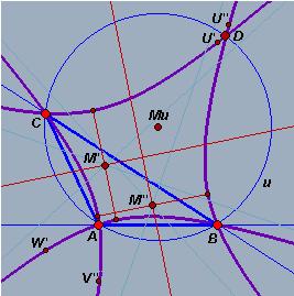
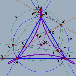
5 Creation of algebraic curves of higher order

The hypocycloid of Steiner, we have seen above, is an algebraic curve of order four. In the special case of an equilateral triangle ABC the two conics c' and c'' coincide with the circumcircle u of the triangle and the Wallace-line [PQR] and the lines [P'Q'R'] and [P''Q''R''] with respect to the point X form an equilateral triangle STU with the following properties, see Fig. 8: The vertex S lies on the circumcircle u of the triangle ABC. The other two vertices T and U describe the same closed symmetrical rational curve of order four with three axes and the three nodes A, B, C. On the other hand the point X always lies on the circumcircle v of the triangle STU and the circumcenter V of triangle STU describes a closed rational curve of order four as well.

These curves we create with Cinderella very quickly using the locus mode with the mover point X. To determine the order of the curves we have to make algebraic considerations by ourselves. The incidence of S with the circumcircle u of the triangle ABC and the incidence of X with the circumcircle v of the triangle STU are automatically reported by Cinderella in the information console.

References

Giering. O. (1998) Seitenstücke der Wallace-Geraden. Österr. Akad. Wiss., Math. naturw. Kl. Abt II, 207: 199-211.

Lockwood, E.H. (1978) A Book of Curves. Cambridge University press.

Richter-Gebert, J. Kortenkamp, J.U. (1999) The Interactive Geometry Software Cinderella. Springer.

Vogel, H. (2001) Use of Cinderella in higher elementary geometry.
http://www-m10.ma.tum.de/~vogel/Cinderella/Klagenfurt

Goto
	Begin of article		Contributions by authors
	Begin of session		Main page

[1] We are talking here of an average family income of under US$ 4000.00 a year for the students in the state school system, and for many teachers as well.

[2] Tabulae were sets of wax filled wooden trays used by ancient Greeks and Romans to jot down messages and diagrams. In other words, an ancient cahier de broullion, or sketchpad!

[3] See www.forum.swarthmore.edu