Working group 4:
Probability simulators and
data analysis programs
Manfred Borovcnik
Klagenfurt, Austria
|
Simulation and modeling with Lisp-Stat |
|
|
Virtual experiments and probability |
|
|
Let the spreadsheet throw the dice—Spreadsheets as |
|
|
Design and use of a computer language for teaching mathematics—Some examples from statistics |
|
|
Improving statistical reasoning: A computer program for high-school students |
|
|
A sample of ideas in teaching statistics |
Tools always influence the ideas behind. Software, initially used to apply statistical procedures, have initiated completely new approaches to statistics, e.g. exploratory data analysis with its open models and interactive modelling, or non-parametric methods with the resampling technique to establish necessary distributions for the comparison of a given set of data, or more recently bootstrap methods.
For the teaching of statistics, it is promising to integrate more realistic problems with the help of data analysis packages – this sheds a better light on the meaning of statistical procedures. The simulation technique gives rise to a material manifestation of quite theoretical concepts like size and power of statistical tests, or simply the meaning of a probability or a probability distribution. Moreover, the graphic capacities of software helps, partially in combination with the simulation technique, to visualize complex ideas like the laws of large number, or the central limit theorem.
For didactical purpose, there are at least two different directions of software for teaching statistics, i.e. as tools for data analysis as a basis for learning environments, and as tools for simulation and modelling. Existing software is quite inhomogeneous: Data analysis tools ranging from procedures from a spreadsheet up to professional data analysis packages like SPSS, either menu-driven or even command-orientated like R or Lisp-Stat; tools for simulation covering single difficult aspects of the curriculum like the distribution of the arithmetic mean, or introducing into the whole chapter of probability and questions of statistical judgement. All in all it holds, the more a software covers from the statistical curriculum, the less it is refined with respect to didactical reflections on how to introduce difficult concepts.
There is an urgent need to specify the requirements of suitable software, or to design guidelines for a fruitful usage of existing, e.g. to make the best sense of spreadsheets, which would have the advantage of wide availability, or to use available hand-held technique to the best in the sense of a didactically refined approach towards the topic.
Such questions were discussed alongside all the presentations in the working group. The single keynote papers were signified by the heterogeneity alluded to previously; they covered the simulation technique as well as learning environments with a command-orientated language. Moreover, the spreadsheet discussion, how far can we come with this popular software, nearly any student has experience with, was taken up.
Joachim Engel and Marcus Otto in their first keynote paper – Simulation and statistical modelling with Lisp-Stat, showed the potential of Lisp-Stat with respect to simulation and statistical modelling; Lisp-Stat has great facilities as a basis but they go together with the burden to learn a specific command language. Maybe it has more advantages if the learning goal is functional thinking, procedural thinking as well as statistical methods. In such a case, the effort pays to overcome the difficult steps at the beginning.
Marcus Otto and Joachim Engel in their second presentation – Design and use of a computer language for teaching mathematics – Some examples from statistics, introduce into a learning environment they created at their university. The focus here is also on using a language for algorithmic reasons and to have a tool for statistics as a by-product which opens all the important topics like a simulative approach to probability distributions, or simulations of statistical tests to understand concepts of statistical reasoning.
Giora Mann’s lecture on – Virtual experiments and probability – discussed advantages and disadvantages of virtual, computer experiments as opposed to hands-on experiments in class. His suggestions were based on Derive – here the twofold goal is to learn this CAS and to get as a reward to understand probability by tackling various probabilistic tasks by simulation programs in Derive.
Erich
Neuwirth followed
quite a different line of approach and argument in his contribution – Let the
spreadsheet throw the dice – Spreadsheets as
Peter Sedlmeier introduced into a learning program – Improving statistical reasoning: A computer program for high-school students, which gives training opportunities to revise wrong ideas about Bayes’ problems and statistical tasks. The special feature of his program lies in a new graphical manifestation of Bayes’ problem, which students should more easily understand than the standard representation by formulae, or by other visualizations.
Piet van Blokland – A sample of ideas in statistics, gave a range of ideas how to use didactic software to enable a better understanding. The situations involved offer a plenty of possibilities to revise misconceptions, he gives incentives for a discussion with the students.
The way to a unique software for all purposes is still a long, better to say, cannot be a goal anymore. The promising aspects of spreadsheets should be clarified, especially in the way how to overcome specific disadvantages of e.g. Excel, which a group under the leadership of Erich Neuwirth is going to do. Learning environments are at the moment under construction at several places, but the hope they will integrate more sophisticated didactical reflections is still to be fulfilled. Application software would gain more space especially for the university education but still there are no reflected guidelines how to make the best profit from them. On the hand-held technology, a lot of efforts have been done in the Standards 2000 and the accompanying ASA-NCTM projects.
Simulation and statistical modeling with Lisp-Stat
Joachim Engel and Marcus Otto
Ludwigsburg, Germany
2. Why teaching statistics with Lisp-Stat?
3. How much is a hair cut? Bootstrap as data recycling
4. Modeling functional relationships between two variables
5. Demonstration of the central limit theorem with Lisp-Stat
We illustrate how a simulation-based use of computers supports conceptual learning in statistics. We focus on three areas of application: bootstrap simulation, modeling functional relationships, and demonstrations of the central limit theorem. The basis is the programming environment Lisp-Stat.
1 Introduction
Teaching approaches to probability and statistics, illustrations of random events and available data analysis methods have changed dramatically over the last two decades thanks to the availability of powerful software and cheap computing power. The use of computers in learning probability and statistics is important for various reasons:
 Enormous computations can be done rapidly: Computers as powerful calculators are a very useful tool for
virtually any mathematical discipline relieving the computational burden and
allowing to focus on concepts, big ideas and strategies for problem solving and
modeling, i.e. everything computers cannot do. Deferring computations to a
machine is not only a mere relief from routine calculations, but constitutes
the basis for modern statistical methods: many recent developments were
unthinkable 30 years ago because they rely on huge computations.
Enormous computations can be done rapidly: Computers as powerful calculators are a very useful tool for
virtually any mathematical discipline relieving the computational burden and
allowing to focus on concepts, big ideas and strategies for problem solving and
modeling, i.e. everything computers cannot do. Deferring computations to a
machine is not only a mere relief from routine calculations, but constitutes
the basis for modern statistical methods: many recent developments were
unthinkable 30 years ago because they rely on huge computations.
Graphical representations and displays can be produced quickly and
interactively: Any exploratory statistics looks for
patterns in data. For this endeavor any interactive graphics software is an
important tool for the data detective, allowing to view the data from multiple
perspectives, to visualize structures in data and to check conjectures by
visual inspection as they incur in the process of exploration.
Data production and management can be done with ease: Mathematical applications live from their relevance to real
problems from the world outside mathematics. Thanks to new technologies like
the Internet current up-to-date data are accessible on almost any subject of
interest. For statistical analysis or calibration of probabilistic models these
data are to be stored, managed, sorted, or transformed: jobs that are hardly
manageable without computers for moderate or large data sets.
Random processes and their laws can be studied experimentally: Some important laws of probability like the law of large numbers,
the central limit theorem or a random walk represented by a Markoff chain are
for many students most convincingly taught through simulations. Similar
considerations hold for the famous three-door-paradox, which had many skeptics
convinced by the change strategy only after a long series of repeated
simulations.
Simulations provide a flexible environment for a wealth of
experiences in stochastic situations: As supported
by recent research (Gnanadesikan e.a. 1997, Hodgson and Burke 2000, Romero e.a.
1995) instruction that incorporates simulation promises to help students
acquire conceptual, and not merely mechanical, understanding of statistical
concepts.
Most problems in probability can be solved either exactly by analytic methods or approximately through simulations. The latter may be the only option available in situations, where the problem is too complex for an analytic approach. Computational Statistics has matured to a sub discipline of its own with numerous international journals and a rich supply of statistical software. A wealth of packages has been developed to address a broad range of special statistical problems. For professional users programs like SPSS, SAS, BMDP and SYSTAT are flexible and very powerful packages. For mathematical statisticians S-Plus as an own object oriented data analytic language has been developed at Bell Labs in the late 80’s. Notable is also its freely available clone R.
2 Why teaching statistics with Lisp-Stat?
Since the early 80's computers have been used for teaching probability and statistics. Even at the school level algorithms have been written in languages like Basic, Fortran or Pascal. Today versatile mathematical software like spreadsheets and computer algebra systems are also available for teaching probability and statistics. Despite their general usefulness do these packages rarely meet the special needs and requirement for probability and statistics instruction? Downscaled professional packages (like Student Systat) differ from their original version only by limited data-processing capabilities. Quite often they provide a multitude of options intended for the professional user, but confusing for the novice. Programs like WinStat, Medass or DataDesk were developed with obvious pedagogical intention. All three programs are relatively easy to use through icons and menu-controlled buttons. They allow interactivity in constructing charts and graphical representations. Data analysis, simulation and modeling, however, are limited to a few functions pre-defined by the program designer. Lisp-Stat is much more flexible in this regard.
Lisp-Stat combines the strength of a general purpose programming language with the needs in data analysis for interactive, experimental programming. Lisp-Stat is based on the Lisp language. The statistical extensions to Lisp consist in large part of Lisp functions modeled on the S respectively S-Plus language (Becker, Chambers and Wilks, 1988) and include basic data-handling functions, sorting, interpolation and smoothing, probability distributions, matrix manipulation, linear algebra and regression. Lisp-Stat includes support for vectorized arithmetic operations, a comprehensive set of basic statistical operations, an object-oriented programming system, and support for dynamic graphics. Lisp-Stat can be used as an effective platform for a large number of statistical computing tasks, ranging from basic calculations to customizing dynamic graphs. The standard statistical graphics in Lisp-Stat include line and scatterplots, histograms and boxplots, scatterplot matrices with brushing, spinning plots and dynamic links between different plots of the same data sets. At a deeper level, the software provides very general access to the underlying graphics system. With advanced skills it is possible to program a wide range of dynamic graphical methods.
The data type that Lisp-Stat is based on, allows manipulation of groups of figures and data sets as whole objects. The same holds for models, i.e. functions, used to describe data. In many cases models can be described by functions or classes of functions. Lisp-Stat allows treatment of functions as objects that can be manipulated by easy commands resulting in new functions, having functions as argument etc. The basic program is lean; the set of available commands is limited, avoiding to distract novices with a multitude of functions and buttons. Lisp-Stat can easily be extended and adjusted to the individual needs of a user.
The Lisp-Stat philosophy is based on lists (LISP= LISt Processing): By
(def temperature (list 21 26 27 31 25 23 27 28 34 37 35 38))
a list of daily temperatures in degree Celsius over a two week summer period is defined. Especially convenient is the application of mathematical manipulations for all elements of a list. With
(def temp-in-Fahrenheit (+ (* temperature 1.8) 32))
the temperature values are transformed into degrees Fahrenheit while
(mean temperature)
computes the mean value of all figures of the list temperature. Computations and manipulations can be applied element wise to whole data sets. Observe here the for Lisp typical and strange prefix notation of mathematical operations which Lisp uses entirely. Another technical feature typical for Lisp-Stat is the high number of brackets: Almost any arithmetic computation is written in brackets.
(log temperature)
results in a list of logarithmic temperatures,
(sqrt temperature)
produces a list of square roots of the temperatures. Random numbers are very conveniently generated. For example, (normal-rand 10) generates a list of 10 realizations of a standard-normal random variable, (poisson-rand 20 5) produces 20 random numbers according to a Poisson random variable with parameter 5.
3 How much is a hair cut? Bootstrap as data recycling
Instead of discussing the syntax and data analysis commands in more detail we illustrate along three examples how Lisp-Stat can be used as an instrument to problem solving, simulation, modeling and demonstration. For the many details of the Lisp-Stat language we refer to Tierney (1990).
How much do students pay for a haircut? A survey of n=15 students resulted in the following figures (in Euro): 20, 0, 15, 0, 32, 24, 16, 15, 64, 0, 10, 17, 25, 31, 18.
Since the hypothetical distribution (of all students) is barely symmetric but rather skewed to the right, we are interested here in the median x0.5 as location parameter: in the example the sample median is 17. This is our estimator for the median of all students. What does this figure tell us? Very little! Each estimator varies. Had we asked a different group of 15 students we most likely had ended up with another estimate. To evaluate the quality of the estimated median of 17 we need information about the distribution of the random variable “sample median of 15 randomly chosen students”.
The classical approach in statistics computes a confidence interval by relying on the assumption that the test statistics (i.e. the sample median) follows a specific distribution, e.g. a normal distribution. Is there reasonable doubt to assume a specific distributional class (like the normal distribution), classical statistics has no answer. This is where the bootstrap method comes in (Efron and Tibshirani 1993). It only assumes that the sample is representative for the population. It is based on the following idea: from the original data x1, x2, …, x15 new, artificial data are generated. More specifically, by drawing with replacement from the set {x1, x2, …, x15}, we generate a new sample of the same size n=15: x*1, x*2, …, x*15 . Here almost always some of the observations are being repeated while others don’t appear at all in the bootstrap sample. From the bootstrap sample we compute again the median. Repeating this procedure (with the computer random generator) over and over again (e.g. b=1000 times) results in 1000 different medians m1, m2, …, m1000 . This procedure is represented in Fig. 1.
It is most instructive to implement the bootstrap algorithm in computer code. A program in Lisp-Stat with the name bootstrap-median that generates b bootstrap medians from a list named data is as follows:
(defun bootstrap-median (data b)
(if (= b 0)()
(cons (median (sample data (length data)t))
(bootstrap-median data (- b 1)))))
|
|
Starting position: sample x1, x2, …, xn |
|
|
|
|
↓ |
← |
↑ |
||
|
draw new sample with replacement |
|
repeat very often e.g.1000 times |
||
|
↓ |
|
↑ |
||
|
Bootstrap sample x*1, x*2, …, x*n |
→ |
compute median |
Fig. 1: Illustrating the bootstrap procedure for the sampling distribution of the median
The logical value t in the command sample guarantees that the drawing mode is with replacement while cons is a constructor producing a list and (sample data n) draws a sample from data of size n.
We take the empirical distribution of 1000 artificially generated bootstrap medians as an approximation for the unknown sample distribution of the sample statistics “median of 15 random values”. Fig. 2 shows a histogram of the medians of 1000 bootstrap samples. What does this result mean? Even if we could draw an infinite number of samples and compute their medians, the resulting sample distribution remains an estimated distribution, which is in itself a random quantity as it depends on the original random sample. The bootstrap procedure can be applied to virtually any statistics of interest. This is very convenient to implement in Lisp-Stat:
|
|
|
|
|
Fig. 2: Histogram of medians from 1000 bootstrap samples |
||
(defun bootstrap (statistics data b)
(if (= b 0)()
(cons (funcall statistics (sample data (length data)t))
(bootstrap statistics data (- b 1)))))
Here statistics is any statistics of interest (like the median in the previous example). For example, a call of
(bootstrap #’mean haircut 500)
produces 500 bootstrap medians from the list haircut and
(bootstrap #’interquartile-range haircut 1000)
produces a list of 1000 interquartile ranges. Provided we stored the list of 1000 bootstrap medians in a list named bs-median, we can now compute any parameter of interest for the empirical distribution of medians, e.g.
> (interquartile-range bs-median)
2
> (median bs-median)
17
> (quantile bs-median 0.05)
15
> (quantile bs-median 0.95)
15
> (standard-deviation bs-median)
3.02533076912695
4 Modeling functional relationships between two variables
We illustrate modeling a functional relationship of two variables with Lisp-Stat. The example we refer is from Simonoff (1995). The data contain monthly average temperatures and average energy consumption of an electrically heated house over a time period of 55 months. The data are stored in two lists: temperature contains the 55 average temperature values, elusage the 55 electrical usage (in Kwh). For a graphical display of the data, we type
(plot-points temperature elusage).
For later reference and interactive dialogue it is convenient to define the plot as a graphical Lisp-Stat object
(def elusage-scatterplot (plot-points temperature elusage)
Even though for the data at hand obviously inappropriate, we first consider linear regression. This is done with the command
(regression-model temperature elusage).
resulting in tables for the coefficient estimates, a summary of fit and an analysis of variance table. To draw the regression line into the scatterplot, we write
(send elusage-scatterplot : abline a b).
where a, b are intercept and slope obtained from above command, in our example a=116.72, b=-1.36. For the current data a nonlinear function characterized by a three-dimensional parameter q seems more suitable, like e.g.
![]()
Estimation of the parameter vector q is based on the Newton-Raphson algorithm (requiring initial estimators) and is conveniently implemented in Lisp-Stat as follows:
(defun f (theta)
(+ (/ (select theta 0 ) (+ temperature (select theta 1)))
(select theta 2)))
Calling
(nreg-model #’ f elusage (list 100 8 20))
results in computing the goodness-of-fit including various summary statistics for the parameter estimates. When starting with above initial values we obtain the estimates q0=4311.49, q1=6.52 q2=-33.57. The fitted curve is added to the plot by (see Fig. 3)
(send elusage-scatterplot :add-lines temperature (f (list 4311 6.5 -33.6)))
|
|
|
|
|
Fig. 3: Scatterplot with nonlinear fit |
||
|
|
|
|
|
Fig. 4: Scatterplot smoother with slider for bandwidth choice |
||
Finally, a nonparametric kernel estimator for the regression curve that does not require specification of a particular class of model functions is easily implemented. Lisp-Stat knows a function called kernel-smooth, which performs kernel estimation based on a bandwidth parameter h (Fig. 4). It sets up a slider allowing an interactive choice of the bandwidth. The final bandwidth then can be chosen by inspecting the different smoothes obtained by moving the slider.
(kernel-smooth temperature elusage)
5 Demonstration of the central limit theorem with Lisp-Stat
Did the last two examples draw our attention away from parametric model specifications and the assumption of normally distributed data; this distribution nevertheless occupies a central position in probability and statistics. Under very general assumptions the distribution of a large sum of independent parts follows approximately a normal distribution. This holds true (almost) entirely regardless of the distribution of the original data. This is the claim of the central limit theorem. In a simpler version it says that sample averages of i.i.d. random variables are approximately normal. An appropriate sample size for this approximation to hold depends largely on the shape of the original distribution. Symmetry here plays a key role. Even when starting with distributions that are markedly different from normal but are symmetric like the uniform, the approximation to the normal distribution is achieved for moderate sample sizes. In contrast, when starting with more asymmetric distributions like an exponential random variable, a much larger sample size is required for the asymptotics to ‘kick in’.
|
|
|
|
|
|
|
|
|
|
Fig. 5: Demo of central limit theorem |
|
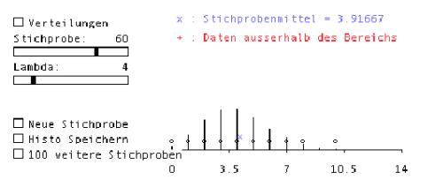
Fig. 5 shows a window generated by a Lisp-Stat macro to demonstrate the Central Limit Theorem (Marasinghe e.a. 1996). In the upper frame the type of distribution and sample size of the original sample is chosen, here: Poisson distribution with parameter l=4, sample size n=60. The lower frame of Fig. 5 shows a histogram including a kernel density estimate based on 501 likewise generated means of 60 Poisson distributed random variables.
6 Summary
Lisp-Stat is a flexible, extensible (and free!) functional programming environment for data analysis, probability and statistics. It has been strongly influenced by S-Plus, but unlike the latter it is based on an existing command driven programming language, namely Lisp. As programming language Lisp-Stat has representations that are close to the formal mathematical language. Whole data sets can be manipulated conveniently as objects.
Important for applications in probability and statistics is the ease and flexibility for simulations and defining arbitrary models. Lisp-Stat has many data analysis functions available. In addition, many macros can be downloaded from the Internet. With these the environment can easily be extended and adapted to the individual needs of its user.
Lisp-Stat is a high-level language, in many ways like S-Plus, but with the advantage that it can get to lower level operations, particular graphics operations. It has only a fraction of statistical operations available that S-Plus has, but the result is a system that is leaner and more transportable. For teaching purposes it provides everything needed in introductory classes of probability, statistics and data analysis. After getting used to the Lisp-specific syntax of prefix notation and bracketing, the basic commands are easy to learn and to remember. They are close to mathematical notations. Nice graphical capabilities are available. They can be customized to special needs and interests, but this requires advanced skills with Lisp-Stat that certainly exceeds what can be expected of students in introductory courses. However, when prepared by the instructor, macros incorporating illuminating graphics may include animation, sliders for choosing parameter values and many more nice features. These then may help students who use these macros as black boxes.
Unfortunately, the online-documentation is very poor. Help consists of two or three cryptic lines that may be a helpful reminder for the knowledgeable user but hardly directs the novice. Also data entry facilities are poor. An environment that is based on Lisp-Stat with an enhanced interface, icons and data management facilities is the program Vista developed by Young(1996).
There is an interesting project at www.omegahat.org. The idea is to develop connections between S-Plus, R, Lisp-Stat so that the user of one program can easily call another without having to know much about that other program. This is nice because Lisp-Stat has some great features that cannot be found elsewhere. That way people can use Lisp-Stat without having to learn it.
7 How to get Lisp-Stat?
Lisp-Stat has been developed by Luke Tierney (University of Minnesota) in the late 80's. In its implementation Xlisp-Stat is based on the Lisp-dialect Xlisp, which had been developed by David Betz, which for non-commercial use is freely available under
http://www.stat.umn.edu/~luke/xls/xlsinfo.html
Many macros can be found in the Xlisp-archive of the University of California (UCLA)
and from StatLib at Carnegie Mellon University in Pittsburgh:
ViSta is available under
http://forrest.psych.unc.edu/research/vista.html
References
Becker, R.A., Chambers, J.A. and Wilks, A.R. (1988) The New S Language. Wadsworth, Pacific Grove, CA.
Efron, B. and Tibshirani (1993) An Introduction to the Bootstrap. Chapman and Hall, New York.
Gnanadesikan, M., Scheaffer, R.L., Watkins, A.E., and Witmer, J.A. (1997) An activity-based statistics course. Journal of Statistics Education 5(1).
Hodgson, T. and Burke, M. (2000) On Simulation and Teaching of Statistics. Teaching Statistics 22, 91-96.
Marasinghe, M., Meeker, W., Cook, D., and Tae-Sung S. (1996) Using Graphics and Simulation to Teach Statistical Concepts. The American Statistician 50, 342-351.
Romero, R. e.a. (1995) Teaching Statistics to Engineers: An Innovative Pedagogical Experience. Journal of Statistics Education 3(1).
Simonoff, J. (1995) Smoothing Methods in Statistics. Springer, New York.
Tierney, Luke (1990) LISP-STAT. An Object Oriented Environment for Statistical Computing and Dynamic Graphics. Wiley, New York.
Young, Forrest W. (1996): Vista: The Visual Statistics System. Research Memorandum 94-1(b). L.L. Thurstone Psychometric Laboratory, Univ. North Carolina.
Virtual experiments and probability
Giora Mann and Nurit Zehavi
Beit Chanan, Israel
This work originated from two classroom activities. The first one took place in Grade 8 algebra class, and the second in a teacher-college probability class. In both cases virtual experiments were performed in response to authentic needs that arose during classroom discourse.
1 Introduction
A game: Warring expressions
Two expressions,
2(x + 6) –2 9 and 7x + 3(1 – x) ,
were given in Grade 8. The students were asked to ‘draw’ 10 integers from –20 to 20 (using the Derive command –20 + RANDOM(41)), to substitute the numbers in the given expressions and to decide on the winning expression according to the higher numerical result. The aim of the game was to lead students to the notion of algebraic inequality (but this is not the story of this paper). Based on the accumulated findings, some students commented that the game was not fair; others said that it was fair since they played with random numbers. Students’ involvement in the fairness issue challenged the teacher to introduce a virtual experiment by preparing a small program using Derive functions.
The probability that a random number is divisible by 3
Students in a teacher college were asked to invent problems in probability similar to those they learned in class. Most of them came up with standard problems, for which they knew the answers. One student invented the following problem:
Each of the digits of a five-digit number is a random number from 1 to 5.
What is the probability that a number generated in this way is a multiple of 3?
The students and the lecturer worked on the problem for a while, and those who thought they solved it got different answers. Some of the students gave an intuitive answer, 1/3, without being able to justify it. Even the lecturer was not sure if he got the right answer. This provoked him to design a virtual experiment by writing a program (in Derive) that models the student’s problem. The experimental result gave a value that was larger than all the answers obtained in class, however a little less than 1/3. This called for reflection on the models used by the solvers that led through refinement to the construction of proper models.
2 Virtual experiments
We will first explain what we mean by virtual experiments (in probability) in CAS environment and then apply it to the two activities described above. A virtual experiment is done by running a program using the random generator of a specific computer language. In this case we use the functional programming of Derive. Clearly, the virtual experiment should model the original problem, like any scientific experiment. The following example demonstrates what we mean by a virtual experiment for a probability problem.
What is the
probability that
while throwing a coin four times one gets two heads and two tails?
Model I: There are five possible results: four heads, three heads and one tail, two heads and two tails, one head and three tails, four tails. Hence, the probability for two heads and two tails is 1/5=0.2
Model II: There are 16 possible results: hhhh, hhht, hhth, hthh, thhh, hhtt, htht, htth, thht, thth, tthh, httt, thtt, ttht, ttth, tttt. Six of these results are successful. Hence, the probability of two heads and two tails is 6/16=3/8=0.375.
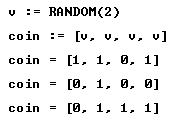
How to decide which is the right model (if at all)? Here comes a virtual experiment. We start by “throwing” a coin four times, by using v:=RANDOM(2). Here one is head and 0 is tail. The name of each trial is “coin”.
|
|
|
|
We can repeat the trial coin any number of times. Let’s repeat the trial 6 times:
|
|
|
|
Only one trial (the first of the six) was successful. Let’s try again:
|
|
|
|
This time we faired better – two successes: the 2nd and the 3rd. Let’s try again:
|
|
|
|
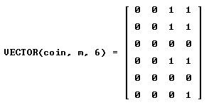
This time we faired even better – three successes: the 1st, the 2nd and the 4th (by the way all three successes were of the same type – tthh).
The next step is to let DERIVE select those trials that were successful:
|
|
|
|
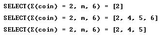
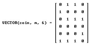
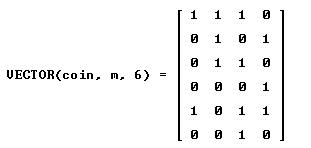
The last three lines tell us that in the first set of six trials only the second was successful; in the second set, the 2nd, 4th, 5th and 6th trials were successful; in the last set, the 2nd, 4th and 5th trials were successful. we add now a command that counts number of successes in 16 trials:
|
|
|
|
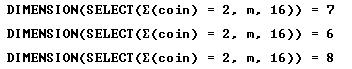
In the first set of 16 trials 7 were successful; in the second set we have 6 successes; in the last set of 16 trials we have 8 successes.
We are ready now to carry out a virtual experiment:
|
|
|
|
We have now good experimental evidence in favor of model II.
A game: Warring expressions
To explore the unfairness of the game the following program was prepared by the teacher and used by the students. In the program a LIST consists of 1000 random integers from –20 to 20. List1 and LIST2 are obtained by substitution of the drawn numbers in the expressions.
|
|
|
|
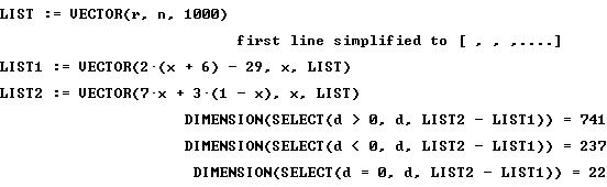
The results obtained by the program can be used in introducing the concept of frequency. The frequency that the first expression wins is 741/1000 which quite close to the actual probability 30/41.
The probability that a random number is divisible by 3
Only very careful counting will result in the right answer for the combinatorial problem: ‘how many of the five digit numbers are divisible by 3. Designing a virtual experiment is much easier. We start by creating random five digit numbers, denoted by ‘a’:
|
|
|
|
Then we create a vector of 10 five-digit numbers:
|
|
|
|
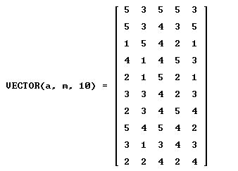
The next step is to create a vector of the sums of the digits of each number:
|
|
|
Now, we look at the vector of remainders:
|
|
|
and then we want to select the 0’s (division by 3):
|
|
|
|
At last we can count the divisions by 3:
|
|
|
|
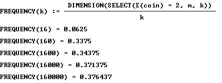
This leads to the definition of frequency:
|
|
|
|
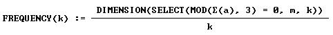
Here are some results of the virtual experiment:
|
|
|
|
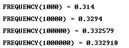
It means that the probability is a little bit less than 1/3. Why can’t it be exactly 1/3? Because there are 55 = 3125 numbers, and 3125 is not a multiple of 3. Now, the first candidate for the probability is:
|
|
|
|
but it seems too big. We try another candidate:
|
|
|
|
So, we have two candidates for the probability. Which is the right one? Careful counting gives the right result – 1041/3125. The virtual experiment led us to an approximate result. But only careful combinatorial calculations gave the exact result!
3 Modelling in probability
A good model in probability must agree with observation, that is: the numeric answer should not be too different from the frequency one observes while repeating the relevant experiment many times. We know that it is not practical to perform the real experiment a great number of times. But, it is very practical to perform virtual experiments in a CAS environment. It means that modelling in probability is changed dramatically by the ability to perform virtual experiments: the student has much better control over his modelling. The frequency he gets from the virtual experiment enables him to reflect on his model. Moreover, the act of designing a virtual experiment is modelling in itself. Once we learned about virtual experimentation, we may say that modelling in probability is twofold – traditional modelling processes controlled by modelling of virtual experiments.
The implication for mathematics education is that programming virtual experiments becomes inseparable from solving problems in probability. After mentioning the benefits of virtual experiments, we should stress that the design of a virtual experiment can go wrong. Therefore some probability model should control it. Moreover, we must remember that the frequencies obtained by the virtual experiment, by their nature deviate from the probability.
Let the spreadsheet throw the dice — Spreadsheets as Monte Carlo simulation engines
Erich Neuwirth
Vienna, Austria
4. More general discrete distributions
Monte Carlo simulation (using computer generated pseudo random numbers) is an extremely helpful tool for illustrating concepts in probability and statistics. It is surprisingly easy (and surprisingly unknown) that this kind of simulation can easily be done with spreadsheet programs. We will show some simple examples from probability and some moderately advanced examples from inductive statistics (testing and estimation) to demonstrate how simulation can help "getting the feeling" for randomness convergence of frequencies to probabilities.
1 A simple example
Modeling throwing coins can be accomplished by generating random numbers taking the values 0 and 1 each with probability 0.5. Let us assume that 1 indicates a head and 0 indicates tail. All spreadsheets have a function RANDOM (or similar), producing real random numbers between 0 and 1 and with uniform distribution on the unit interval. Therefore, the formula =IF(RAND()<=0.5,1,0) produces the desired random number. Copying this formula down a few hundred times repeats the experiment.
In what follows we refer to special properties of Microsoft Excel. Other spreadsheet programs might have the same behavior, but in some cases it also might not be possible to have the same recalculation behavior.
Calculating the sum of this column gives the number of 1s and therefore the number of heads in our series. Dividing the number of 1s by the total number of experiments (=number of rows with our formula) gives the relative frequency of heads in our simulation. The formula we are using is a “live” formula, whenever a worksheet is recalculated, all the formulas generating random numbers are recalculated and will produce new random numbers. Excel recalculates each time function key F9 is pressed, so the relative frequency of our series of experiments is recalculated each time F9 is pressed. Therefore, this very simple spreadsheet models repeated execution of a series of random experiments.
2 Extending the example
In the next step, we want to model throwing dice. So we need an integer random number between 1 and 6. =6*RAND()produces a real random number in the range 0 to 6, therefore rounding down gives an integer random number in the range 0 to 5, and =INT(6*RAND())+1 produces random numbers between 1 and 6, all with probability 1/6.
To calculate relative frequencies, it is very convenient to use Excel’s built-in FREQUENCY function. This function is slightly difficult to use since it is an array function. Array functions have results too large to fit in one cell, they have “array values”.
The formula is set up in the following way in Fig. 1.
|
|
|
Fig. 1 |
The marked regions with the numbers indicate the input areas for the cell, and the marked region with the formula indicates the output region for the formula. To create an array formula, one has to select the output area before entering the formula, and one has to press Control-Shift-Enter instead of Enter when the formula is finished.
Like in the previous example, Pressing F9 recalculates the random numbers and therefore produces a new frequency table. Using spreadsheet graphs, a histogram can be created visualizing the frequency distribution, ant then pressing F9 each time produces a new histogram. Repeating this often gives a visual display of random fluctuations of histograms from empirical data.
3 A more complex example
In the next example we will repeat series of 10 coin flips and calculate the number of heads in each series. Using the formula of the first example can accomplish this, but we will modify the example to be able to deal with unfair coins also.
|
|
|
|
Fig. 2 |
Fig. 3 |
Fig. 2 shows how to create a formula modeling an unfair coin. The formula to the right of 1 has to be copied down far enough, then the column with the formula models the repeated coin flips. The value 0.6 in this worksheet is the probability of getting heads, so changing this we can model different coins.
Calculating the sum of this column gives the number of heads in a series of 10 coin flips.
To repeat this experiment in the spreadsheet we will “creatively misuse” the Data Table menu command. Data Table in its simplest application takes values from one column one by one, puts these values in a preassigned cell, and records the value of another preassigned cell.
Fig. 3 shows the layout we need to be able to use Data Table. We created a column with sequence numbers for the repetitions of our experiment, and next to it one row above we created a formula indicating the cell “to be watched”. Selecting the area shaded gray and using the Data Table command from the menu, and indicating an empty cell for Column input cell in the dialog box of this menu command creates the repetitions of our experiment.
Now we can use the frequency function and create the frequency table and the histogram for this experiment. We can vary the probability of heads and study the histograms. Pressing
F9 again recalculates the whole spreadsheet. In our case this implies that the whole series of experiments (each experiment being a sequence of “atomic” experiments) is repeated and the frequency table and the histogram is recalculated.
4 More general discrete distributions
So far we have modeled two types of discrete distributions: binary distributions with arbitrary probabilities and multi-valued distributions with equal probabilities. Using nested IF statements we could produce arbitrary multi-valued discrete probabilities, but there is a more elegant way.
Let us create a formula producing random numbers according to the following table (Fig. 4) i.e. 1 with probability 0.4 and so on. We can accomplish this by first creating a column of “running sums” of the probabilities next to the probabilities.
|
|
|
|
|
|
|
|
Fig. 4 |
|
Fig. 5 |
|
We use this table (Fig. 5) in the following way: We now produce an intermediate uniformly distributed random number between 0 and 1. If this number lies between 0 and 0.4, our final random number is 1. If the intermediate number lies between 0.4 and 0.5, our random number is 2 and so on. The Excel function LOOKUP implements this algorithm. LOOKUP take 3 arguments. The first one is a single number (the lookup value), the second one and the third one are columns of equal length. The function finds the closest value in the first column smaller than or at most equal to the lookup value and returns the value from the second column as the result of the function call. This is exactly what we need. Combining LOOKUP and RAND allows us to produce arbitrary discrete distributions.
5 Summary
We have tried to demonstrate that some rather basic techniques allow us to create Monte Carlo simulations of practically every discrete distribution of reasonable size. We need rounding functions, if-functions, and a uniform real 0-1 random number generating function. For the more advanced examples, we need Data Table and LOOKUP, and FREQUENCY. This toolkit is sufficient for a wide range of Monte Carlo simulation.
In our paper we did not discuss the quality of the random number generator. Random number generators in standard office programs like Excel usually are not very high quality. Therefore, one has to be careful about the interpretation of the results. Additionally, discussion about the relationship between simulations and “real” random experiments are important and always should follow simulations. The examples described in this paper (and possibly some more) are available from
http://sunsite.csd.smc.univie.ac.at/Spreadsite/montecarlo/
- Further spreadsheet information is available on this Web site.
References
Neuwirth, E. and Arganbright, D. Spreadsheet Programs as Tools for Mathematical Modelling, in preparation.
Neuwirth, E. Recursively defined combinatorial functions: Extending Galton's board. Discrete Mathematics 2001 (to appear).
SunSITE Austria Spreadsheet resources, http://sunsite.univie.ac.at/Spreadsite/
Design and use of a computer language for teaching mathematics —
Some examples from statistics
Marcus Otto and Joachim Engel
Ludwigsburg, Germany
During the last years, we designed a computer language and used it in mathematics education. Our aim was to establish a tool for learning and doing mathematics. The language can be shaped to meet the needs of a course. Besides using such a language for algorithmic purposes, one can create its own mathematical structures based on their features, relations and operations. Students can use this to investigate the concepts presented in a course. Taking concepts from probability and statistics as examples, we illustrate how to incorporate our language into mathematical teaching.
1 Introduction
At the Pädagogische Hochschule Ludwigsburg our primary concern is to educate/train the next generations of math teachers. We are convinced that computers play an increasing role in mathematics and math education. More than a decade ago we started to use computer languages in several courses. To better meet our needs, we then decided to design our own language.
We found that a main reason why schoolteachers don’t use computers is that they lack own experience in using computers as a tool for doing mathematics. They rarely developed the concepts of how calculators and computers work and how they represent mathematics. Algorithms, for example, often aren’t made explicit or even discussed formally. Also mathematical representations are optimized for the convenience of writing and reading. There should be more concern about how to represent a problem in such a way that a machine can solve it.
2 Design goals
It is our goal to develop a computer language, which doesn’t force the instructor to focus too much on machine-oriented representations, but give him/her the freedom to use own terms and formulations. Therefore, the language should be flexible and scalable.
Desiderata:
We
need a language, where it isn’t necessary to declare whether 16 or 32 bits
represent our numbers, but where we can use rational numbers with no
(noticeable) size restrictions.
The
names of operators should be chosen in analogy to the names used in mathematics
and their semantics should be what we expect from a mathematical point of view.
Also, operators important for working on mathematical problems should be
provided.
Furthermore,
the teacher should be able to change the names of operations to whatever he/she
decides to use in his/her course. There shouldn’t be the need for using
different names for the same thing, getting students confused. Or even worse,
using a wrong name because it is set by the language for historical reasons or
whatever.
It’s
also important, that the teacher is able to extend the set of operations
provided by the language. It should be possible to add shortcuts and black
boxes to make the use of the language in the course easier.
There are more design goals like easy handling, support for graphical representations, use of external code (java applets for example) that we don’t discuss here.
3 The computer language LUCS
Our language LUCS (LUdwigsburger ComputerSprache) is based on the Lisp dialect Scheme, which was introduced in 1975 at the MIT. Since then it has been developed to incorporate modern concepts and is now widely used around the world, especially for educational purposes (see Kelsey, Clinger and Rees 1998 and Abelson and Sussmann 1996). Our main reasons for choosing Scheme are: its simplicity (completely defined in fifty pages, based on five basic commands), the elaborated concepts (for example a complete number tower including rational and complex numbers), and its extendibility through a macro mechanism. Our implementation is based on Kawa, a Scheme interpreter programmed in Java (see Bothner 2001). This gives us access to many of the features of the Java platform including object-oriented programming and sophisticated user interface functionality.
Besides a handy user environment (see figure 1), we added several new features to LUCS. These include:
facilities
to adapt and extend the language. This covers infix and postfix notations,
including precedence rules. Also provided are the definition of shortcuts or
aliases, as well as new data structures and the use of keywords to identify
function arguments.
native,
math-based names for almost all language features. This includes language
constructs for ‘handling cases’ (Fallunterscheidung) and ‘where clauses’
(wobei).
additional
mathematical functionality provided through various extension packages. They
comprise different fields such as linear algebra, analysis, elementary
geometry, graph theory and others.
The two main rules in using the language are: a) white space matters and b) the function symbol goes within the parenthesis. For example, a simple term like a + b ´ c writes like (a + b*c) and the application of the sine function to p is written as (sin pi); 3/4 denotes the rational number that is the result of the expression (3 / 4).
|
|
|
|
|
Fig. 1: The user environment of LUCS during a regression calculation |
||
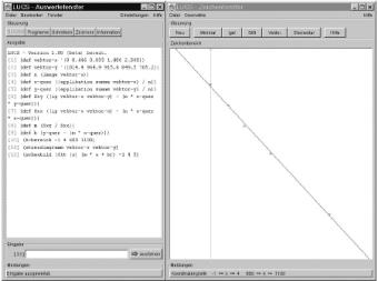
LUCS is a functional-applicative language, i. e. it is based on defining functions and applying them to values.
(def (f x) (x ˆ 2))
(f 5)
Þ 25
The evaluation order is applicative, which means that the arguments are evaluated before they are inserted into the function body. This is in contrast to the behavior of functional languages like Haskell (see Jones and Hughes 1999), which use lazy evaluation (though we are able to provide such an mechanism as well).
As with its ancestor Lisp, we use the list as a main data structure in LUCS. This gives us a handy tool, especially when dealing with sequences of data, as it is the case in statistics.
(def temperature ’(21 26 27 31 25 23 27 28 34 37 35 38 33 31))
A quote is used to handle an expression, as it is, i. e. it prevents evaluation. We added some higher functionality for list processing, for example to make it easier to handle repeating operations on lists (see Shivers 1998 and Jones and Hughes 1999).
Though we believe that the prefix notation of Scheme is very valuable through its simplicity, most of our students had problems with it. We therefore introduced infix and postfix notations and also precedence rules to LUCS (this goes along with other functional languages like Haskell (see Jones and Hughes 1999).
4 Use in statistics
In a course about probability and statistics LUCS can be used in different ways. On the one hand, one can investigate basic concepts by formalizing them in a computer language and then applying them in various ways. On the other hand, one can leave a lot of the number crunching to the machine, which allows more extensive explorations on the subject.
When looking for places and ways to integrate LUCS in teaching, one should keep this in mind:
Whenever
writing a formula think about an equivalent LUCS definition.
Whenever
thinking about a formal representation of a concept think also about a
representation as a data structure in LUCS.
Do
not restrict the use of LUCS to algorithms, though they are a good point to
start.
Do
concentrate on basic concepts and write simple functions. Do not try to provide
a handy user interface and a colorful visualisation from the beginning.
If
a concept you deem important is missing in the language, try to add it. Shape
your own language that meets your needs and fits into your course.
Do
not try to change everything in one day. Start with simple add-ons or
replacements and develop these incrementally from one course to the next.
Next, we give some examples for using the LUCS language in a statistics course. We provide them in their original German form to show the similarity to common and native language.
Statistical measures
An easy point to start with are those basic statistical functions that are defined by a simple one line formula. For example, the mean could be defined as follows:
(def (mittelwert liste)
((summe-der-elemente liste) / (anzahl-der-elemente liste)))
It is on you to decide whether you give this definition to the students or use it as a black box. You may even give them the following definition.
(def (summe-der-elemente a)
(falls
(gilt (a leer?)
dann 0)
(sonst
((summe-der-elemente (a ohne-letztes)) + (letztes a)))))
It is similar to the mathematical definition of the sum, given in the following formula:
This works for a lot of basic concepts like median and quantiles. Other examples are standard deviation and interquartile range. Let your students do some of the definitions. Let them explore and find out about the nuts and bolts of these concepts.
Probability distributions
Probability distributions are an example of a concept that can be represented by a data structure. We can write discrete distributions as lists of element-probability pairs (written as lists of two elements respectively).
’((e1 p1) (e2 p2) ...)
To support this structure we then define accessor functions like getting the i-th event of the distribution or the list of probabilities.
(def (ites-ereignis i v)
(erstes-element (i tes-element-von v)))
(notiere-infix ’tes-ereignis-von ’ites-ereignis)
(def (liste-der-wahrscheinlichkeiten v)
(bildliste zweites-element v))
Based on this we are able to define the probability of a list of events by:
(def (ereignis-wahrscheinlichkeit e-liste v)
(summe-der-elemente
(liste-der-wahrscheinlichkeiten
(auswahlliste ((x)->((erstes-element x) enthalten-in e-liste))
v))))
Random numbers
A central topic of statistic courses are random numbers. With the following definitions students are able to generate and explore random numbers and discuss the problem of “calculating” them.
(def (kongruenzfunktion a b m)
((x) -> ((a * x + b) mod m)))
(def (kongruenzliste n anfangswert kong-fkt)
(falls
(gilt (n = 0) dann ’())
(sonst
(anfangswert vorne-an
(kongruenzliste (n - 1)
(kong-fkt anfangswert)
kong-fkt)))))
The first definition gives us a function constructor, i. e. its result is a function (l-expression) that maps x on (a´x + b) mod m.
The second definition states a function to generate a list of pseudo-random numbers. It takes the size n of the list, the starting number (seed) and the congruence function as arguments and calculates the list by the following recursive formula:
k-list (n, z0, f) = (z0, z1, ..., zn-1)
where
(z1, ..., zn-1) = k-list (n-1, f(z0), f)
Using these functions students are able to experiment with different values of m, a, b, z0. Example:
(kongruenzliste 10 19 (kongruenzfunktion 22 6 50))
Þ (19 24 34 4 44 24 34 4 44 24)
Or using the values of the random generator of DERIVE:
(kongruenzliste 10 123456789
(kongruenzfunktion 3141592653 1 (2 hoch 32)))
We are now able to take an arbitrary discrete distribution, as given above, and generate random elements according to that distribution.
(def (zufallsstichprobe n v)
(falls
(gilt (n = 0) dann ’())
(sonst
((zufallswert v) vorne-an
(zufallsstichprobe (n - 1) v)))))
(def (zufallswert v)
((i tes-ereignis-von v)
wobei
(i steht-für
(position (zufallszahl-zwischen 0 1)
(kumulative-wahrscheinlichkeiten v)))))
The function ‘kumulative-wahrscheinlichkeiten’ gives us the list (F0, F1, ..., Fm), where
![]()
The application of ‘position’ returns the index i for which a random value 0 £ x < 1 complies with Fi £ x < Fi+1.
Simulations
LUCS provides a convenient way to deal with simulations. Being introduced to the following base function for a simulation, our students can design their experiments as LUCS functions and then perform various simulations with them.
(def (simulation n exp)
(falls
(gilt (n = 0) dann ’())
(sonst
((exp) vorne-an
(simulation (n - 1) exp)))))
As before, this definition states that a simulation of size n of an experiment exp is a list. This list contains the result performing the experiment once at the beginning, followed by the results of a simulation of size n-1.
The students now have to define their experiments as functions with no arguments. Let us look at an example from “Activity-based Statistics” (Scheaffer et al. 1996). Given the following scenario, the students were asked to perform randomization tests. The aim is to tell whether the difference between two proportions is statistically significant.
Scenario:
In 1972, 48 male bank supervisors were each given the same personnel file and asked to judge whether the person should be promoted to a branch manager job that was described as “routine” or the person’s file held and other applicants interviewed. The files were identical except that half of them showed that the file was that of a female and half showed that the file was that of a male. Of the 24 “male” files, 21 were recommended for promotion. Of the 24 “female” files, 14 were recommended for promotion. (B.Rosen and T.Jerdee (1974), “Infuence of sex role stereotypes on personnel decisions”, J. Applied Psychology, 59:9–14.)
Our students now had to define a LUCS function that models that experiment. One solution is to start with the modelling of the files. The files will be represented by their main characteristic “male” or “female”. We then produce two lists with 24 files “male” and “female” respectively and then put them together.
(def akten ((wiederholungsliste 24 ’männlich)
(wiederholungsliste 24 ’weiblich) zusammengefügt))
The experiment is then described as drawing a sample of size 35 (the persons promoted) without replacement and calculating the frequency of the males among them.
(def (beförderungs-experiment)
(häufigkeit ’männlich
(stichprobe-ohne-wiederholung akten 35)))
Asking the computer for a simulation of size 100 by:
(simulation 100 beförderungs-experiment)
and drawing a simple line plot students can discuss the results and the value of the method. To support this process they can perform other experiments given similar scenarios (as mentioned in Scheaffer et al. 1996).
(strichliste (simulation 100 beförderungs-experiment))
14 | xxx
15 | xxx
16 | xxxxxxxxxxxxxxxxx
17 | xxxxxxxxxxxxxxxxxxxxxx
18 | xxxxxxxxxxxxxxxxxxxxx
19 | xxxxxxxxxxxxxxxxxxxxxx
20 | xxxxxxxx
21 | xxxx
5 Conclusions
We presented our computer language LUCS and showed its use in probability and statistics. The reasons for using computers and especially computer languages in such courses are stated in Engel and Otto (2003). Designing and using a special language was motivated by the desire to have a tool shaped and shapable to our needs, i. e. to make it fit our course and the concepts and notions used there. We wanted to reduce the overhead given through machine dependent representations and non-native command names.
We gave examples showing how such a computer language can be integrated into a statistics course. From our experience, we found that the use of a computer language supports an exploring style of learning. It provokes discussions about how to model and represent problems. It also supports the students in stating and reasoning conjectures.
Further information about LUCS can be found at
http://www.ph-ludwigsburg.de/mathematik/forschung/schemel/lucs/
References
Abelson, H.; Sussman, G. (1996) Structure and Interpretation of Computer Programs. MIT Press.
Bothner, P. (2001) The Kawa Scheme system. http://www.gnu.org/software/kawa/
Engel, J.; Otto, M.(2003) Simulation and Statistical Modeling with LISP-STAT. (this volume)
Jones, S.; Hughes, J. (eds.) (1999) Haskell 98: A Non-strict, Purely Functional Language.
http://www.haskell.org/onlinereport/
Kelsey, R.; Clinger, W.; Rees, J. (eds.) (1998) Revised5 Report on the Algorithmic Language Scheme. ACM SIGPLAN Notices 33, No. 9, Oct.
Otto, M. ( ) LUCS Homepage
http://www.ph-ludwigsburg.de/mathematik/forschung/schemel/lucs/
Scheaffer, R. et al. (1996) Activity-based Statistics. Springer.
Shivers, O. (1998) Scheme Requests for Implementation 1: List Library.
http://srfi.schemers.org/srfi-1/
Improving statistical reasoning:
A computer program for high-school students
Peter Sedlmeier
Chemnitz , Germany
The TIMS (Third International Mathematics and Science) study has revealed that German as well as American high school students show severe deficits in many areas of mathematics, including probability theory (Baumert et al., 1997). This is consistent with results from psychology research: Adults show poor performance in tasks that deal with judgment under uncertainty, that is, with probabilities (e.g. Kahneman, Slovic & Tversky, 1982). In the area of judgment and decision making the still-dominant view holds that difficulties in adequately dealing with uncertain information – sometimes termed “cognitive illusions” – are as resistant to training attempts as are visual illusions (Gigerenzer, 1991). However, increasing evidence shows that this need not be so: If the tasks that yielded such poor results are changed only slightly, the solution rates go up considerably (e.g., Gigerenzer et al., in press). Tasks have to be presented in a way that invokes pre-existing valid intuitions, that is, spontaneous tendencies to judge or to act in a certain way. It has been shown that whether there is a match between a task and a corresponding intuition makes a big difference in whether things of daily use, such as stoves, doors, light switches or flight schedules, are easy to use or not (Norman, 1988). The use of intuitions has also been explored in mathematics education. Consider the following example from Fischbein (1994):
Problem 1: From 1 quintal of wheat, you get 0.75 quintals of flour. How much flour do you get from 15 quintals of wheat?
Problem 2: 1 kilo of a detergent is used in making 15 kilos of soap. How much soap can be made from 0.75 kilos of detergent?
It turns out that Problem 1 is much easier to solve for 5th graders than Problem 2, although mathematically the solutions are the same. The difference lies in whether one multiplies 0.75 by 15 as in Problem 1 or whether the multiplication is 15 times 0.75 as in Problem 2. Problem 1 conforms to the intuition that if a number is multiplied, it gets bigger whereas Problem 2 contradicts this intuition.
The computer program described here accompanies a textbook on probability theory for German high school students (Sedlmeier and Köhlers, 2001) and exploits just these pre-existing correspondences between valid intuitions and probability tasks. Large parts of the program have been tested successfully in empirical studies (Sedlmeier, 1999, 2000; Sedlmeier & Gigerenzer, 2001). The success of the training program was due to two ingredients: the use of suitable representational formats and learning by doing. Representational formats that are close to everyday life are more likely to evoke valid intuitions than are very abstract ones. In the case of probability theory, this means that if the information in probability tasks is given in frequencies, these tasks are much easier to solve than if the information is given in probabilities, which are quite new in human history; also, if one experiences random sampling or can perform it oneself, probability tasks are solved more easily than if one only reads about random samples (Sedlmeier, 1998). Learning by doing is realized in the program by allowing the users to manipulate graphical interfaces and solve tasks on their own, guided by the program’s feedback.
An example illustrates how the program works (for a more thorough description see Sedlmeier, 2001). Consider the following problem:
A reporter for a women's monthly magazine would like to write an article about breast cancer. As a part of her research, she focuses on mammography as an indicator of breast cancer. She wonders what it really means if a woman tests positive for breast cancer during her routine mammography examination. She has the following data:
• The probability that a woman who undergoes a mammography examination will have breast cancer is 1%.
• If a woman undergoing a mammography has breast cancer, the probability that she will test positive is 80%.
• If a woman undergoing a mammography does not have breast cancer, the probability that she will test positive is 10%.
What is the probability that a woman who has undergone a mammography actually has breast cancer, if she tests positive?
This problem was solved correctly by less than 10% of participants, experts (medical doctors) and laypeople alike, in several studies. The usual way to solve it is to apply Bayes’ formula
p(cancer) = 0.01, p(pos | cancer) = 0.8, and p(pos | no cancer) = 0.1,
as given in text;
p(no cancer) can be calculated as 1 – p(cancer) = 0.99:
If participants are taught how to extract the relevant information from texts and how to use it in the formula, there is some training effect right after the training, but it is almost completely gone one week later. This way of solving a probability revision problem (the probability of a woman having breast cancer is revised in the light of a positive test result) does not seem to evoke any valid statistical intuitions.
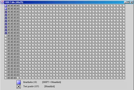
How does the program deal with problems of this kind? It offers two representational formats, the frequency grid and the frequency tree. Fig. 1 shows the solution of the mammography problem with the help of the frequency grid.
From a random sample of 1,000 women, 10 (1%) can be expected to have breast cancer (“Brustkrebs”) and are coloured in Fig. 1. From these 10, 8 (80%) can expect a positive test result (marked by a cross in Fig. 1) but from the remaining 990 women, also 99 (10%) can expect such a positive result. The sought for conditional probability of breast cancer given a positive test result is just the number of women who have cancer and are tested positive divided by all the women with a positive test result: 8 / 107 = 0.075. When participants received a frequency-grid training, the high immediate training effect (about 90% correct solutions in probability revision problems not used in the training) was found to remain stable in retests up to three months afterward.
|
|
|
|
|
|
Fig. 1: Frequency grid |
|
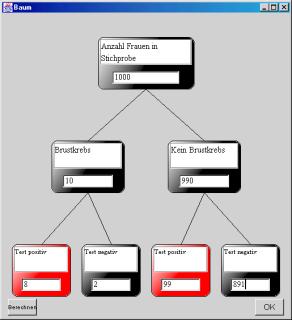
Basically the same result was obtained with a different kind of frequency representation, the frequency tree (Fig. 2). Again, a random sample of 1,000 women (top node in Fig. 2) is divided up into women with and without breast cancer (two middle nodes) and these are divided up into women with and without a positive test result (lower nodes). Again, it suffices to divide the result in the left lower node (number of women with breast cancer and positive test result) by the number of all women with a positive test result.
|
|
|
|
Fig. 2: Frequency tree |
Fig. 3: Probability tree as used in the training studies |
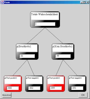
However, one could make the point that the formula training differs from the frequency training also in another respect: non-graphical vs. graphical representation. Do the graphics play a crucial role? This question was examined in a study that compared the frequency tree to a probability tree (Fig. 3). The probability tree is equivalent to the frequency tree except that now numbers are confined to values between 0 and 1 – otherwise calculations remain the same. There is, however, a dramatic difference in training success between the two kinds of representational formats: Whereas both formats yielded comparable short-term training effects, the long-term effect for the probability tree was as low as that achieved with the formula (Sedlmeier & Gigerenzer, 2001).
The computer program also contains an animated frequency representation, the “virtual urn,” that makes random sampling visible. The virtual urn can be filled with all kinds of discrete (population) distributions with the events represented as balls marked with colours and symbols that can be chosen freely. The animated sampling procedure can be performed with and without replacement. The virtual urn is the basis for all simulations in the program. It could be shown empirically that the use of the virtual urn helps considerably in understanding and solving probability tasks (Sedlmeier, 1999). The computer program covers all aspects of basic probability theory treated in German high schools, including confidence intervals and significance tests for binomial distributions.
References
Baumert, J., Lehman, R. u.a. (1997). TIMSS—Mathematisch-naturwissenschaftlicher Unterricht im internationalen Vergleich: Deskriptive Befunde. Leske & Budrich, Opladen.
Fischbein, E. (1994). The interaction between the formal, the algorithmic, and the intuitive
components in a mathematical activity. In R. Biehler, R. W. Scholz, R. Strässer, &
B. Winkelmann (eds.) Didactics
of mathematics as a scientific discipline. Kluwer,
Gigerenzer, G. (1991). On cognitive illusions and rationality. Poznan Studies in the Philosophy of the Sciences and the Humanities 21, 225-249.
Gigerenzer, G., Hertwig, R., Hoffrage, U., and Sedlmeier, P. (in press). Cognitive illusions reconsidered. Plott, C. R. and Smith, V. L. (eds.) Handbook of experimental economics results. North Holland/Elsevier Press.
Kahneman, D., Slovic, P., and Tversky, A. (eds.). (1982). Judgment under uncertainty: Heuristics and biases. Cambridge University Press, New York.
Norman, D. A. (1988). The design of everyday things. Doubleday, New York.
Sedlmeier, P. (1998). The distribution matters: Two types of sample-size tasks. Journal of Behavioral Decision Making 11, 281-301.
Sedlmeier, P.
(1999). Improving statistical reasoning: Theoretical models and practical
implications. Erlbaum,
Sedlmeier, P. (2000). How to improve statistical thinking: Choose the task representation wisely and learn by doing. Instructional Science 28, 227-262.
Sedlmeier, P. (2001). Statistik ohne Formeln. Borovcnik, M. Engel, J. and Wickmann, D. (eds.) Anregungen zum Stochastikunterricht. Franzbecker, Hildesheim, 83-95.
Sedlmeier, P., and Gigerenzer, G. (2001). Teaching Bayesian reasoning in less than two hours. Journal of Experimental Psychology: General 130, 380–400.
Sedlmeier, P., and Köhlers, D. (2001). Wahrscheinlichkeiten im Alltag: Statistik ohne Formeln. Westermann, Braunschweig.
A sample of ideas in teaching statistics
Piet van Blokland
Amsterdam, The Netherlands
Probability and statistics is a broad subject. Software can help in several ways to enhance the teaching of statistics and probability in secondary education. It can help to illustrate the use and importance of probability and statistics in society. It can help to show how close statistics is to the daily life of the students. Software can help to clarify some misunderstandings or illuminate some concepts. It is important to realize that statistics and probability is more then only a part of mathematics.
1 Broader content
Statistics is much more then a part of mathematics. Some basic concepts of statistics like the difference between an observation and an experiment and the importance of randomised comparison experiments are not mathematical of nature. Moore (1997) has pointed this out in many articles. Mathematics education tends to emphasize too much on theoretical probability and all kind of counting problems. A good sample of questions how to start a course different is given by the questions from www.planetque.com by Harris (2002).
1 What is 'luck'?
2 What is the biggest risk you have taken today? This year? In your life? When and why do we "leave it to chance"?
3 What are the different ways in which humans cope with chance?
4 What are the current developments in the human reaction to the world of chance?
5 Where does risk come into our daily lives? Is the way we perceive/react to risk independent of context?
6 How much do you know about the risks that are 'managed' for you by governments and other organizations and of the 'methods' they use?
7 What is meant by the terms independent events and cause and effect? How are they related?
The questions asked here, show the importance of the subject and connect the subject more to the emotional side of students. Statistics and probability does often play an important role in questions about medical treatment, gambling, politics etcetera. It should be part of general education to understand some of the questions involved in these issues.
2 Polls
Polls are one of the easy way’s to do statistics with students. Proper wording, biased sampling are important questions to consider if polls are made. Students should have software at hand, which is easy to handle. The students should put their attention to the real questions involved and that should not be how to handle this or that program. There are several packages, which are simple enough for secondary school students. An aspect to consider “multipoint questions”. These are questions, which allow more then one answer. For example, if students are asked about there leisure activities (Sport, reading, dancing, etcetera) it is possible that they do more then one activity. If students are asked to make there own opinion poll, these multipoint questions arise naturally. Most statistical packages demand that these multipoint questions be split up in several questions. This is not so easy to explain and afterwards to analyse such questions becomes even more troublesome.
3 Sampling
Statistics has some contra-intuitive results. It turns out that the idea of sampling is very difficult. How is it possible with a random sample of 1000 to get a reasonable reliable estimate of the percentage of pro-voters of 240 million Americans. Even if students know how to calculate the confidence interval, they do not really believe the results.
“De nationale doorsnee” is an experiment in the Netherlands where 50173 students of the age 12 to 13 participated. At one day in 2000 whole classes spend some time to fill in a questionnaire and send the results to a website. The questionnaire contained questions about weight, length, work, and pocket money etcetera. The whole dataset of 50173 records is now available for statistical education. Now students can take easy samples out of this huge dataset and compare the results of several small samples. A question to investigate is “When is the sample large enough to do a reliable statement?
One of the things that can be shown in the huge dataset itself is the prevalence of multiples of five when asked about length or weight. This phenomenon cannot be show at the small dataset. Another misunderstanding with students is that if the sampling method is not right it does not help to make the sample larger. In the huge dataset the percentage of boys is 48,87% while according to the statistics of the CBS (census office in the Netherlands) the percentage of boys is 51.10%. The sample of 50173 students is biased. First students should be asked for reasons of this bias. (Maybe boys are more ill then girls, or they more often absent at school, or .. .) Then they are asked to take samples and to investigate if larger samples give a better result.
4 Simulations
Simulation is one of the most promising ways to use software in the classroom. Hands-on activities are natural. Students make there own data. Realistic situations can be investigated. The simulation No-show, Fast food service, Monopoly, One-armed bandit, “I predict you” will be discussed.
No-show: No-show simulates that several passengers of an airplane do not show up at the time the plane leaves. This gives huge costs to airplane companies. Sometimes airplane companies oversold the number of chairs. No-show is an example to show the practical usefulness of simulation. It turns the view of the student from himself to the eyes of the company. Therefore, it does help giving real meaning to question 6 of planetque
Fast food services: Fast food service shows the effect of a waiting line. Students can change the number of possible customers that walk by, the number of servants and the number of possible customers that walk through if they see a waiting line. The output of the simulation is the number of customer served, the number of possible customers not served, the time personal worked and the time personal did not work because of lack of customers. This simulation too turns the eyes of the student to the eyes of the owners of the company.
One-armed bandit: Gambling plays an important role in our society. A lot of money is involved in the gambling industry. Education should teach something about concepts involved with that. A lot of money is earned from our young students. Many students will face the problem of gambling addiction in their life. The fruit machine simulation is made with one big idea behind it. It is all right when you play, but it will cost you money in the average.( About 20 euro each hour). If you think that this is a lot of money for standing behind a stupid machine then you should not play. If a fellow student comes with big stories how much money he has won, students who have used this simulation have stronger arguments against his claims. Of course simulations do not stop gambling addiction but it should make it a subject to talk about.
“I predict you” is only a simple example of a program with the purpose of explaining students the way intelligent programs predict their behaviour. The student is asked to type 40 zeroes and ones in random order. The software has the power to analyse this sequence. It assumes that there is some regularity in the random sample the student typed. If a student typed after three 000 usually a 1, the computer uses this knowledge to predict the next key.
5 Testing hypothesis
What a hypothesis and the alternative hypothesis really mean, is a difficult question in school. Quite a lot of concepts are involved: The value of the parameter, the alfa, the observation, the left, right or both sided formulation of the hypothesis, the critical region, the p-value. On the graph below you can see that students can influence all these values and look to the results of changes immediately. Besides that the formulation of the test is shown. It shows the students that the working out of a hypothesis is a mechanical process, even a computer can do.
|
|
|
|
|||
|
|
Fig. 1 |
|
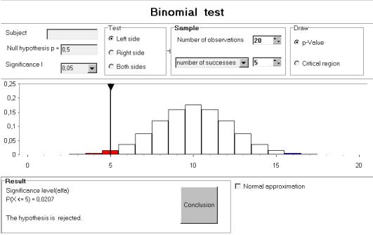
6 The central limit theorem
This is a demonstration program. Whatever skewed distribution is started with, if enough independent draws are made, the sum of all these independent distributions is close to a normal distribution. It is those little tricks of easy filling in a skewed distribution, which make software easy to handle if you are demonstrating in front of a classroom.
|
|
|
|
|
|
|
Fig. 2 |
|
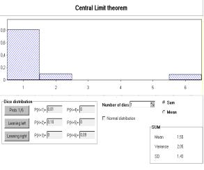
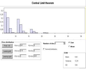
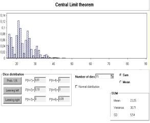
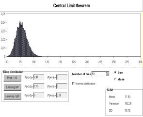
7 Quality control
This is a subject that in my opinion is important for students. Not from the mathematical point of view, but as a way that our society uses to improve its production of goods and services. It is now used on so many places that students should know about the philosophies behind it. (Deming). If someone has an idea of software that let students create data, improve the process and discover in this way the philosophy and methods of quality control I am very eager to program it.
References
Harris, D. (2002) www.planetqhe.com
Moore, David S.(1997), New Pedagogy and New Content: The Case of Statistics, International Statistical Review 65,123-165.