Working Group 1:

Computer animation, visualization,

and experimental mathematics

Gert Kadunz

Klagenfurt, Austria

Douglas Butler	Adding a sparkle to classroom teaching — Introducing Autograph
Kate Mackrell	The role of dynamic geometry packages in visualization and animation
Susanne Saminger	MeetMATH — Visualizations and animations in a didactic framework
Ralf Schaper	Mathematica graphics in the Internet: Additional lighting and clipping in LiveGraphics3D
Grosio Stanilov Lidia Stanilova	Mittels Computer zu mathematischen Entdeckungen
Yulian Tsankov	Cubic section by moving plane

1. The presentations within the working group

2. Some fruitful questions for the future

3. Conclusion

Visualization of mathematics is a far land. At ICTMT 5 we could see that “Computer animation, visualization and experimental mathematics” has developed even further than the presentations in our working group suggested. The lectures covered interesting topics from maths education and production of learning environments to the presentation of theorems of geometry. Beside these contents new software for doing mathematics was demonstrated and solutions for software errors were offered.

1 The presentations within the working group

D. Butler’s (Oundle School, Peterborough, UK) report on Autograph provided an incredible amount of software features from the first to the last minute of his lecture. Nearly all school mathematics and even several parts of mathematics at university level can be explored with his software Autograph. Combining text, formulas, diagrams, and the interactive manipulation of them were the highlights of Mr. Butler’s presentation. In his words, he added a sparkle to the classroom.

K. Mackrell, UK, presented numerous interesting examples from Cabri software focusing on the role of dynamic geometry packages in visualization and animation. These comprised not only geometrical examples, but also some examples of calculus and algebra.

G. Stanilov (University of Sofia “St Kliment Ohridski”), an experienced mathematician, offered an approach to use the computer to investigate mathematical problems.

The starting point of Mr. Stanilov’s colleague, Y. Tsankov, asked for cutting a cube with a moving plane. The informative presentation of his solution was supported by the use of images generated by Mathematica.

R. Schaper from the University of Kassel, Germany, well-known for his book “Grafik mit Mathematica”, showed solutions for Mathematica software errors in his presentation on Mathematica graphics in the Internet.

S. Saminger (University of Linz, Austria) introduced a family of interactive courseware –MeetMath. Her presentation focussed on a fruitful combination of ideas on visualization and animation within a didactic framework with the new technologies.

2 Some fruitful questions for the future

Regarding the metaphor of a far land for the visualization of mathematics, all of these presentations offered a lot of research work for the future. Some of the questions might be:

What is the task of an experiment within mathematics education?

Why should we teach all these beautiful examples in school mathematics? Are there other reasons to teach them beside their beauty?

How can teachers offer their experiences to software developers? Is it necessary to implement more and more features? How can we use software in everyday school?

What are the main features of visualization if we look at visualization in a more sophisticated way? Can we answer such a “simple” question like “What is an image?”

3 Conclusion

We are positive that the working group “computer animation, visualization and experimental mathematics” offered a variety of examples for doing mathematics, thinking of maths education and developing tools. For the future there will be enough material for doing research in two directions, developing tools and examples for mathematics in school on the one hand side, and doing research work in the field of psychology, epistemology and pedagogy to help our students to learn mathematics on the other hand side.

Goto
	Begin of article		Contributions by authors
	Begin of session		Main page

Adding a sparkle to classroom teaching

– Introducing Autograph

Douglas Butler

Peterborough, UK

1. Autograph

2. Sample lessons using Autograph

3. Conclusions

1 Autograph

Autograph is a new program that takes the world of dynamically linked objects into coordinate geometry and statistics. It has evolved over years in the classrooms at Oundle School, Peterborough, and has recently been professionally programmed in C++ by Mark Hatsell.

Fig. 1

Autograph has a powerful mathematical notation entry system, which accepts fully implicit expressions right up to 2nd order differential equations. Equation entry is by single-line text, so expressions can be copied and pasted easily (e.g. from an email or a word document). Whereas dynamic geometry systems operate in the Euclidian plane and have just 3 ‘primary’ objects (the point, the line and the circle), Autograph operates with 6 primary object types:

In the x-y coordinate plane (or r-θ):
Equation (Cartesian, parametric, polar, 1^st2nd order differential)
Bivariate Data set (a single object representing the set of points)
Single coordinate points (free moving, or attached to curves)
Group of points (forming a shape that can be moved about/transformed)

In the single-variable probability and statistics environment (f-x or p-x)
Grouped data set (with or without raw data)
Probability distribution (uniform, binomial, Poisson, geometric, normal, user defined)

Dependent objects can be created from these; animation is generated by dragging than object, or by varying constants and parameters.

This paper is concerned with how these animations can be used effectively in the classroom to enhance visualization and understanding. A static paper is not the ideal medium for this, so the animations will have to be left to the reader’s imagination! Links with Word and Excel are achieved seamlessly by using standard formats (bit-maps, meta-files, comma-separate data and text). The web site, www.autograph-maths.com, offers support for teachers with

data sets; links to useful web sites and internet data sources;

sample Autograph, Word and Excel files – these are all small files users can download the appropriate application and run the files from the web page. This technique is being used to support the web-based Further Mathematics course in the UK.

2 Sample lessons using Autograph

Sample lessons on various topics

The most effective way to use Autograph in the classroom is with a screen that the pupils can all see, and one, which you can write on with a white-board marker (e.g. a TV or, a projector displaying on a white board). All these examples form part of the “45 Exercises”, recorded as ScreenCam demonstration, available for download on the Autograph web site.

Transformations A perfect dynamic situation: the original objects can be moved around, and the parameter that created the second object can be animated. Write on top of the images on the while board to get the students to anticipate the results before the computer.
	Fig. 2
Transforming curves Illustrated here is: y = x², and y‑b = (x – b)² and then vary a and b. Using function definitions works well too, e.g. plot f(x) = x², then y = f(ax+b) + c and vary a, b, c. Then redefine f(x) as sinx.
	Fig. 3
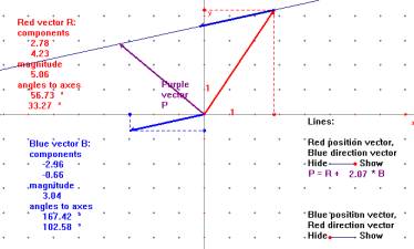
Fun with vectors The principle of copying, adding and subtracting vectors can be explored dynamically. Also scalar multiples (vector equation of a line). The difficult concept of a unit vector can be explored by constructing a unit circle over it and varying the parent vector.
	Fig. 4
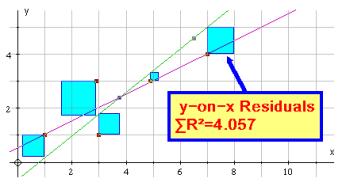
Illustrating residuals Here a variable line is constructed through the centroid and another random point. This line and the data set (which is an object) are selected and the y-on-x residuals illustrated as square. Vary the second point to watch the squares minimize.
	Fig. 5

Sample lessons on the principles of calculus

There are many aspects of calculus that can be taught much more effectively with dynamic images. The old thought that a picture is worth a thousand words is never more true, and students gain new insights by observing movement through animation, driven either by the teacher in ‘whole-class’ presentation, or by themselves working through instructions in a lab.

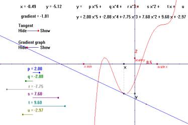
The concept of gradient (a) Zooming in on the gradient of a chord as x2 => x1, observing Δy = 0 and Δx = 0 yet Δy/Δx => 2. (b) Autograph can draw the gradient function slowly, and users can dynamically move a tangent along the parent curve.
		Fig. 6
y = 1/x and e and y = lnx This lesson first shows, by varying the right limit of the area under y = 1/x to find e.Then plot y = lnx, and show that its gradient is the right branch of y = 1/x. Then develop an argument for y ‑ ln(‑x) and finally y = ln|x|
	Fig. 7
Numerical methods Solving equations by Newton-Raphson, and by the x = g(x) iterative method both lend themselves perfectly to a dynamic approach. The start point can be dragged around, and the equations can have variable parameters.
		Fig. 8
Differential equations Here is a lesson showing the principle of the complimentary function and particular integral. The implicit form of the entry allows the RHS to be changed, say, to sinx. Also, the original equation can have a variable parameter, e.g. y’ + ky = x.	y’ + y = x y = x –1
	Fig. 9

Sample lessons on probability and statistics

Frequency density It is useful to be able to plot a set of grouped data so that students can see the difference between representing the data as discrete (displace to the left) or continuous, and by frequency or frequency density.
	Fig. 10
Poisson approximation Students can get a good insight into the relationship between a binomial distribution and its Poisson approximation by varying the binomial’s n and p. Hypothesis tests on the binomial can also be illustrated dynamically.
		Fig. 11
Data off the net The data for the UK Lottery (6 balls from 49) is collected from all previous results and downloaded to Excel. The distribution of the first ball (in order) copied to Autograph offers an unusual bar chart, box and whisker and cumulative frequency diagram.
		Fig. 12

3 Conclusions

There are many issues and challenges to meet when expecting teachers to use dynamic software in their teaching. There are rich rewards, but hardware, content and training issues all need to be addressed. Teachers need to be convinced that the investment in time is worthwhile, and budget holders need to be convinced that mathematics is a subject that needs ICT investment. The author would be glad to hear from anyone who feels this battle is being won, against a background of worsening teacher shortages, and declining interest in mathematics amongst school pupils. Technology can help, but it cannot replace teachers!

Goto
	Begin of article		Contributions by authors
	Begin of session		Main page

The role of dynamic geometry packages in visualization and animation

Kate Mackrell

Brighton, UK

1. Introduction

2. What are the capabilities of dynamic geometry?

3. How do we achieve our aims?

4. Ways forward

This session comprised a report of discussions held at the CabriWorld conference in Montreal in June 2001 regarding the use of Cabri-Geomètre to create interactive teaching materials using visual imagery and animation to introduce mathematics from a wide range of areas.

1 Introduction

It is currently very difficult for ordinary teachers to create their own software, particularly software that uses the facilities of a Windows environment, which means that many creative ideas simply cannot be implemented. One possible solution to this problem is the use of packages such as Cabri-Geomètre or Geometer’s Sketchpad. Materials exploiting the excellent animation possibilities of these packages can be devised to use in mathematics teaching across the curriculum. One example of such materials is Active Geometry, created by the Association of Teachers of Mathematics in the U.K. This consists of Cabri or Sketchpad files and text containing activities related to the files that enable students with no knowledge of Cabri or Sketchpad to work in areas directly related to the English national curriculum, such as transformations, straight line graphs and area as well as traditional geometry. Following on from the Active Geometry project, I have created materials for use across an even broader range of topics, from number and algebra to handling data. There are a number of issues involved in creating such materials and, in order to introduce some of the techniques which can be used (email me for details) and to further explore the issues involved I conducted a series of sessions at the CabriWorld conference in 2001. Much of the following is a synthesis of ideas expressed at this conference.

2 What are the capabilities of dynamic geometry?

Fundamentally, anything that involves visual imagery can be effectively explored using Cabri (or any of the other DGS). The following is a description of files, which illustrate the wide range of mathematical topics, which can be approached. These can be downloaded from http://www.cabrikate.com/.

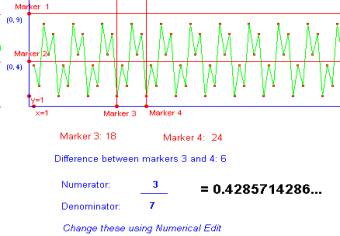
Number Enables the exploration of recurring decimals via a graph of the decimal digits. Fig. 1

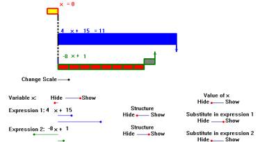
Algebra A concrete representation of algebraic expressions which can be used for exploring the meaning of variables, expressions, substitution and solving equations. Fig. 2

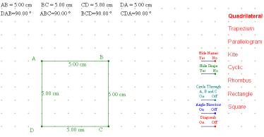
Traditional Geometry (from Active Geometry) As the student manipulates the vertices of a quadrilateral, different names appear which describe the shape. Fig. 3

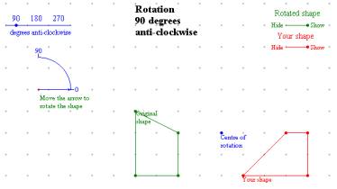
Transformations (from Active Geometry) Enables prediction of the effects of various rotations Fig. 4

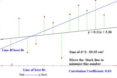
Statistics To explore regression and correlation. Data points can be moved and a line can be dragged to fit the data. Fig. 5

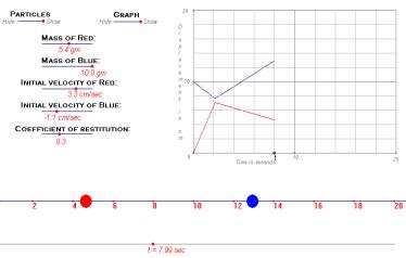
Modelling 1 Two balls collide and a displacement-time graph is drawn Fig. 6

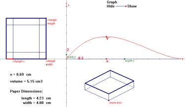
Modelling 2 The Maxbox problem: What is the largest open-topped box you can make from a sheet of paper? Three linked representations of the situation are given. Fig. 7

Calculus A graph in which a point on the x axis may be animated to demonstrate dy/dx, or d²y/dx². Fig. 8

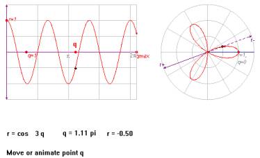
Polar graph A link of Cartesian and polar graphs to explore rose curves. Fig. 9

Vectors Vector equation of lines with 2D vectors Fig. 10

It is also useful to consider the different aspects of mathematics that we want students to learn – each of which may require different types of pedagogical intervention. Mathematical knowledge may be considered as facts (the “arbitrary”, Hewitt, 2001), skill and understanding (the “necessary” Hewitt, 2001).

Facts: for example the Active Geometry quadrilaterals file enables students, by finding out when the names “quadrilateral”, “cyclic” etc appear as the figure is changed to learn about the concepts underlying the various names at the same time as encountering the names.

Skill: There are various ways in which skill can be considered.

Straightforward “lower level” mathematical skill: for example the Active Geometry rotation file will enable students to practice rotation

Visualization: students’ ability to internally represent mathematical situations is enhanced by experience manipulating these situations in a dynamic environment.

Ability to use Cabri-Geomètre: The learner needs very little knowledge of Cabri to make effective use of these files but the full capabilities of Cabri are available and hence the files may serve as a starting point in learning to use Cabri.

Higher-order mathematical thinking skills: We want learners to be able to look at a situation, ask questions, make and test conjectures, generalise and explain why generalisations hold true. Many of the files (such as the polar graph) form “micro-worlds” which can be explored in this manner.

Understanding is a major aim with the files: many were designed to illuminate specific concepts, such as the file in which equations of lines are given in vector form.

One aspect of the files which can aid understanding of these is the linking of different representations of a situation, as occurs in both the modelling files, where a picture of the situation is linked to a graph and with the polar graph, where different graphs are linked. Another aspect is the use of animation to create motion. In the calculus file watching y change as x moves can give a dynamic understanding of what differentiation is all about. Cabri can also enable an entirely new understanding of a concept. Dynagraphs enable students to move away from the concept of a function as a machine that inputs and outputs numbers to gain an understanding of the behaviour of a function. Here is an illustration: as the point x is moved, the point f(x) moves.

Fig. 11

It is an open question whether or not Cabri can contribute to student learning in the area of proof. It’s certain that the “microworlds” files are amenable to students asking and answering the question “why” and there exist excellent demonstrations of well-known theorems designed to aid student understanding. I refer people to Hans-Jürgen Elschenbroich’s paper in this volume: my website also contains examples based on his ideas. Another excellent example is the file Pythag that comes with Cabri. Another possibility is to sequentially show the steps of a formal proof.

3 How do we achieve our aims?

As Ros Sutherland says, the evidence is that students do not automatically engage with mathematical software: the teacher must “craft the culture”. Teacher-centred learning can be positive: questions can be asked and activities devised that will engage a class when working with only one computer (Alison Jeavons gave an exciting account of the use of Sketchpad in just such a manner at ICTMT 5) — but it can also be negative: students do not automatically learn and understand from demonstrations.

The alternative possibility is for the learner to take control and work independently with a file. Many people felt that the learner must have control in order to learn effectively. Hans-Jürgen Elschenbroich made a distinction between multimedia, where learners remains passive and didactic visualization in which learners need to act. I distinguish two types of control. The first of these is control by construction, in which the learner explores a mathematical situation by constructing objects. The second type of control is control by manipulation, in which a learner manipulates objects, which they may or may not have created. In many situations both types of control are achieved: the learner first constructs objects and then explores them to study their behaviour.

Control by construction is necessary for the formulation stage of mathematical modelling. Students may also prefer to work with objects they themselves have constructed: for example students with no knowledge of Cabri preferred to use spreadsheets they constructed themselves to explore recurring decimals rather than the Cabri file supplied to them. However, constructing with Cabri can be problematic: to paraphrase Hans-Jürgen Elschenbroich, starting with a blank screen is lengthy and error-prone and pre-prepared worksheets avoid the learner needing to engage in “geometrical programming”. Construction and manipulation may also have different learning outcomes: I learned very little by creating the polar graph (and nothing about rose curves)– but learned a great deal about the behaviour of rose curves by manipulation.

An interactive teaching file gives control by manipulation: how can we best ensure that students will take control and that this control will lead to effective learning? We need to first consider the type of manipulation. Paul Goldenberg stressed the importance of actual hand movement in manipulation, because of the enormous amount of information we thus receive. All manipulation of basic Cabri objects (apart from numbers) involves hand movement, but we have a choice about how we enable changes to numbers: it may be important to create sliders rather than use Numerical Edit.

The next issue is how we get students to engage with the files. Some students stare at a file blankly while others have the mathematical maturity to approach a file, pose their own questions and learn for themselves. Some files (such as the polar graph) are more engaging than others. However, for a large number of learners and situations it is important that the files are supplemented by materials containing activities designed to engage the students.

A selection of activities from Active Geometry can be found on either the CD ROM version of these proceedings or on my website. Some of these activities are straightforward, but many questions are geared toward developing higher-order skills: the learner is asked to find out what is happening and to explain why it is happening. Some questions lead to open-ended exploration, while others are puzzles to be solved. However, teachers only feel a sense of ownership when they design their own activities. A teacher who wrote about her successful experience of using Active Geometry in the classroom (Gibbons (2001)) designed her own task and did not use the activities provided. On the other hand, I have seen trainee teachers stare blankly at Active Geometry files, having no idea what they could do with them. It would hence seem important to include activities to give teachers ideas of what is possible but to make sure that there is scope for modification and the creation of new materials.

Here are a few further comments:

A file should be visually appealing.

Files and activities should be designed together.

The design of a file should take very careful account of common misconceptions. I once created a file in which a ladybird travelled parallel to the y axis, at the same time as a graph was drawn of its motion. On testing this file, a student perceived the ladybird as travelling up and down, just as the graph went up and down, thus reinforcing the misconception that a travel graph represents a trip up and down a mountain!

We must ensure that answers to the question “why” are accessible to learners and that maths is comprehensible rather than “magical”. This may mean making files far simpler and less visually impressive than we would like.

We must be open to students exploring aspects of the situation that were not intended by the creator of the file: these explorations may be of more value to the student than our intended learning outcomes.

We need to consider what we potentially lose when we make use of ICT. An example is the “maxbox” file. If this file is used on its own, students miss the formulation phase of modelling and the opportunity to select appropriate approaches to the problem. Given an actual piece of paper, I have seen students come up with creative possibilities, such as the box “with a basement” (formed out of the four squares cut out of the corners).

A question: is there a chance that too perfect an external representation might get in the way of constructing an internal representation of a mathematical situation? I once gave a lesson which involved particular patterns on a number square. I used “good” materials: hundred squares, OHP transparencies, etc. Another teacher however had used no materials and had only written a few snatches of a number square on a blackboard. The incompleteness of this representation propelled her students into using algebra in a way that few of mine had come anywhere near.

4 Ways forward

During the coming academic year, I will be engaged in a research project which will involve developing further materials and trialing materials in a number of schools. I would welcome feedback from any teachers who would like to use any of the materials in their classroom. I will also be creating materials to facilitate teacher (and potentially student) learning of aspects of Cabri that may be useful in developing such files.

Active Geometry for either Geometer’s Sketchpad or Cabri-Geomètre is available from the Association of Teachers of Mathematics, www.atm.org.uk

References

Proceedings of CabriWorld 2001.

Gibbon, J. (2001) Some lessons using dynamic geometry software. Micromath 17(2), 39-40.

Hewitt, D. (2001) Arbitrary and Necessary: Part 2 Assisting Memory. For the Learning of Mathematics 21(1).

Goto
	Begin of article		Contributions by authors
	Begin of session		Main page

Visualizations and animations in a didactic framework

Susanne Saminger

Linz, Austria

1. Introduction

2. From teachers to learners

3. Didactic rooms

4. Visualizations and animations

5. Concluding remarks

MeetMATH denotes a family of interactive mathematics courseware produced within the scope of the initiative „New Media in Education on Universities and Colleges“ of the Austrian Ministry of Education, Science and Culture. The didactic framework and basic concepts of these products have been developed during the project IMMENSE (Interactive Multimedia Mathematics Education in Networked universities for Social and Economic sciences) of a consortium led by the Johannes Kepler University Linz, Austria and the Austrian Ministry of Education, Science and Culture.^[1] Main aspects of the didactic concept^[2] will be presented as well as the resulting challenges for the technical development of courseware and their realization within MeetMATH.^[3]

1 Introduction

Similar to society the perception of education has changed - life-long learning is no longer an idea but a necessity. Concepts for training and education, especially with respect to electronic learning materials (eMaterials) and electronic courses (eCourses) have to be adapted or even changed from the traditional training situation „somebody teaching in the front - somebody learning in the back”. A reflection on learning objectives has to take place not only in the cognitive area, but also on the affective/emotional and behavioural sector^[4], since goals of the latter two have often been transported as a kind of „hidden curriculum“ in the traditional training situation. Due to the fact that self-paced learning supported only by some eMaterials lacks the human intercommunication and interaction of a teacher in person, developers of eMaterials have to consider at least the following questions:

Which learning objectives should be achievable with specific eMaterials?

Which target group should be addressed?

How to deal with learning objectives, which are not achievable by eMaterials or within an eCourse?

How to design a learning process, which does not concentrate on a teacher or which is not guided by a teacher, but by the learner him- or herself?

Concerning the question of learning objectives, which can not be achieved within an eCourse, the following must be considered: Self-paced learning supported by eMaterials is a specific learning environment. Single learning environments can be extended to learning arrangements by combination with further, additional learning environments, such as tutorials, lectures, discussion boards, etc., whereas one learning environment, e.g. self-paced learning, remains the leading element in the whole learning arrangement. Therefore human intercommunication and interaction might be integrated into the learning process so that further learning objectives can be achieved. The last question might be rephrased in the following way, as it has been of the leading records throughout the development of MeetMATH: „If our aim is to help students to become competent, autonomously acting experts in their field of practice, we must give them the opportunity to behave competent and autonomous as learners too.“

2 From teachers to learners

In the classical, teaching situation teacher control and guide the activity of learners: first they dispose them for new knowledge, then they confront them with new objectives, afterwards the learners practice their new skills or apply their newly acquired knowledge and in the end there is an achievement control. If learners should behave autonomously within their learning process and should guide themselves through it, different tools and corresponding „didactic rooms“ must be provided within an eCourse supporting them in this intention. E.g. they need tools such that they can recognize different learning objectives to be relevant and/or interesting for themselves and tools helping them to finally achieve those objectives. They basically need to know which goals can be achieved by doing a certain eCourse or by doing only parts of it and they need a possibility to determine their lacks of skills and knowledge.

The consequence of didactic rooms is that learning units of an eCourse are an arrangement of different sections, each of them belonging to a didactic room, where learners are free to choose the sequence and the duration of their stay in one of these on their own responsibility. Basically four types of didactic rooms can be distinguished: motivation, confrontation, strengthening and assessment. In the following these four didactic rooms and their challenges for development of eMaterials (on a conceptual basis as well as in respect to technical design) will be discussed.

3 Didactic rooms

Motivation

The main question concerning motivation is: „What is the reason for learners to think about certain facts or to achieve certain competences?“ The answer to this question is as individual as each learner him- or herself. Since there is no possibility within eMaterials to react spontaneously on the learner's needs, many different, optional possibilities must be offered to approach a certain objective. Motivation rooms must be accessible in an easy way, but the attendance at these rooms must be optional. Therefore movies (illustrating real-life problems), animations (presenting complex situations), sounds (reminding of certain situations in everyday life), pictures (showing typically situations), examples and experiments should be optional. Nobody wants to be motivated, if there is no need for motivation and the necessity and interest to deal with a certain topic already exists. From a technical point of view two approaches can be distinguished for making motivational rooms optional in eMaterials. One possibility is to structure a learning unit within an eCourse in such a way that motivational rooms can be skipped, e.g. by using hyperlinks or by clicking a button which makes those parts invisible. The second possibility is to separate motivation rooms and make them accessible through hyperlinks. These links might have a certain style (colour, size, icons, text, ... ) to demonstrate their purpose and to gain a certain announcement effect.

Realization in MeetMATH: Both possibilities have been realized. The different learning units are structured into themes and belong to two main categories: RealWorld and MathWorld. Learners can choose whether their first approach to a certain topic is more based on an application to a real-world problem or is based on a more mathematical point of view (looking at mathematics first might be motivating for learners too, not only if they have to achieve special objectives for an exam!!). Each learning unit starts with a list of learning objectives, which will be treated, and the Mathematica^®-commands used for a „quick solution“. Furthermore there is a description of the central problem of the learning unit and in the RealWorld-units there are also short movies to visualize these problems.

Confrontation

The central concepts must be presented in a complete and carefully paced argumentation. The learners should get the possibility to add new knowledge to their existing knowledge base. In case their knowledge is lacking relevant information to comprehend every part of a new topic, additional rooms might be necessary and can be provided, not to explore the newly gained knowledge, but to fill missing links in the learners' pre-knowledge. The learners can visit the additional parts whenever they think there is a need for more basic details. Within confrontation rooms relevant information, thoughts and illustrations must be offered in a way, such that students are able to build up their own ideas and concepts and/or to modify existing, incorrect concepts.

Realization in MeetMATH: A high value has been set on complete and well paced argumentation. A few cycles of didactic and conceptual reviews have been applied as well as experiments with students of business and economy have been carried out in order to verify and confirm the perceivability of learning units within MeetMATH. Interviews and tests at the end of these experiments have shown that the „quick solution“ of real-life problems by using Mathematica supports the understanding of the underlying mathematical concepts. Furthermore links to so-called „tools“ were inserted in different learning units, which contain additional information about mathematical concepts and should help learners to deal with existing insufficiencies in their pre-knowledge.

Strengthening

Strengthening rooms need to be designed in order to verify, elaborate and consolidate newly developed concepts and ideas. Different aspects of a certain concept can be investigated. Experiments and interactive elements enable learners to verify and stabilize concepts, which have been developed correctly during confrontation. Those experiments also allow them to falsify incorrectly developed concepts or parts of concepts by trial and error. The problems and experiments can differ in detail, structure and complexity, such that there are different possibilities to strengthen the newly gained knowledge. Both, success and failure are possible and allowed during strengthening. Failure indicates that return into a room of confrontation might be necessary. The level and the design of strengthening parts must be considered well, such that strengthening rooms do not degenerate into „rooms of frustration“. Experiments and problems should be understandable and solvable.

Realization in MeetMATH: Strengthening rooms have been realized as parts of a learning unit but also as separated rooms accessible via hyperlinks. Interposed multiple-choice questions have been inserted into learning units for strengthening. Interactive experiments were implemented as interactive Mathematica dialogs, such that a new notebook is opened after pushing a button. Within these experiments different parameters can be changed by the learners by clicking into a graphic or by specified input interfaces. The results or consequences of the changed parameters are shown immediately as text, graphics, Mathematica output, etc. Buttons leading to strengthening parts have been labelled in an explicit way, so that learners get an impression what will happen after pressing the button --- Will a graphic be inserted? Will an animation be shown? Will an interactive experiment be opened? Therefore learners can choose which kind of experiment, better to say which kind of strengthening room they want to enter.

Assessment

Assessment is a necessary tool for supervising a learning process. Since the learners are responsible for their learning process and their knowledge development, they need some tools for measuring their progress and/or for finding out their status quo. Therefore a possibility to assess the newly gained knowledge in order to get a qualitative feedback must be integrated into an eCourse. A test, carried out in an assessment room, will consist of different questions. The design of these questions highly depends on the learning objectives, which should be achieved within the specific eCourse.

Realization in MeetMATH: Assessment rooms have been designed as separated rooms. There are three different possibilities to assess one’s knowledge: generating a test for a certain learning unit, generating a test for a topic, generating a test for the whole eCourse. In the first case learners can choose specific questions by clicking buttons, in the second and the third case the number of questions for the test can be chosen, which will be selected from a question pool by chance. The feedback for a test contains information, whether a single question has been answered correctly or incorrectly or has been answered at all. Additionally qualitative feedback is given and links are provided automatically for linking to the correct learning unit.

The power of Mathematica can on the one hand be used for generating parameters by random. Therefore two learners can work on the same type of question, but the exercise specification contains different coefficients. On the other hand Mathematica can be used to evaluate the learner's answer. Not only multiple-choice-questions have been realized within MeetMATH, but also questions with blank input interface, e.g. an empty placeholder.

4 Visualizations and animations

Before going into details the meaning of „visualization” and „animation” have to be considered since there are different concepts in mathematics didactic.^[5] On the one hand „visualization” is used for expressing the graphical representation of mathematical contexts and for the process of illustrating (basic) terms of mathematics. On the other hand „visualization” is associated with the interaction of learners with pictures and/or graphics, which foster and facilitate the acquisition of concepts, proofs or problem solving strategies. Both concepts of visualization are integrated into MeetMATH.

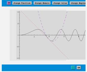
In the first sense the power of Mathematica has been used for generating plots and graphics of certain mathematical contexts and terms, e.g. two-dimensional functions, inequalities, etc., see also Fig. 1. The second concept has been realized by interactive experiments (as already mentioned in section 3). Only a few impressions of some of the implemented experiments can be shown in the following figures. Fig. 2 shows an interactive graphic concerning the objective function within a feasible region at the beginning and at a possible end of an experiment. Learners influence the situation just by clicking into the graphic. Fig. 3 shows the interaction possibilities through specified input interfaces within an experiment concerning Taylor series of a function.

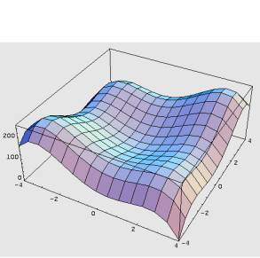
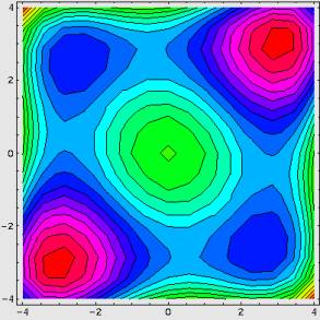
Fig. 1: Mathematica-plots of a two-dimensional function

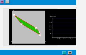
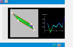
Fig. . 2: Interactive experiment: Objective function within the feasible region

Animations differ from visualizations in the sense that there is no interaction possibility for learners except for starting and quitting the animation. So animations are fixed sequences of certain graphics or pictures. Movies have been integrated which illustrate a given real-life problem. There are also animated graphics showing a mathematical context, e.g. move of the objective function over the feasible domain. Visualizations and animations play an important role for learners in discovering new aspects of a certain, mathematical problem and in intensifying newly acquired and developed concepts. Both - visualizations and animations - will also have a motivational impact on the learning process. Therefore didactic rooms such as „motivation" and „strengthening" are most suited for holding such parts within an eCourse.

Fig. 3: Interactive experiment: Taylor series of a function

5 Concluding remarks

In this paper the concept of didactic rooms for eMaterials and eCourses has been introduced. The four basic rooms - motivation, confrontation, strengthening and assessment – have been presented in detail as well as their realization within MeetMATH. Furthermore the aspect of visualizations and animations within MeetMATH with respect to the didactic rooms has been discussed.

Acknowledgement: The support of the Austrian Ministry of Education, Science and Culture, which fully financed the project IMMENSE, is gratefully acknowledged.

References

Becker, G.E. (1991) Planung von Unterricht. Handlungsorientierte Didaktik. Beltz, Weinheim.

Kadunz, G. (2000) Visualisierung, Bild und Metapher. J. Mathematik-Didaktik 21, 280—302.

Volkert, K.T. (1986) Die Krise der Anschauung. Eine Studie zu formalen und heuristischen Verfahren in der Mathematik seit 1850. Vandenhoeck & Ruprecht, Göttingen.

Goto
	Begin of article		Contributions by authors
	Begin of session		Main page

Mathematica graphics in the Internet:
Additional lighting and clipping in LiveGraphics3D

Ralf Schaper

Kassel, Germany

1. Introduction

2. Problems

3. Solutions to problems

4. Applications

5. Outlook

1 Introduction

Since 1997 Martin Kraus from Stuttgart develops LiveGraphics3D. This is a Java 1.1-Applet to display and to rotate three-dimensional graphics in HTML pages produced by Mathematica. The project is supported by Wolfram Research, especially in showing polytopes. There is also a short user manual. In his well written documentation Martin Kraus mentions two restrictions:(i) "LiveGraphics3D does not clip primitives which are outside of the PlotRange.(ii) In some situations the color of the wrong face of a polygon is used. The reason is the simple (but fast) algorithm being used to decide which face is painted." Two years ago I worked with LiveGraphics3D and I found some solutions. Now at last I will give a short description. Additional information and the Mathematica-notebook you may get from this page.

Initialization

Don`t be alarmed that seven packages will be loaded now. Further on working with this notebook will become easier with these packages. Some hints about installation are given below. Only ExtendGraphics`Geometry3D` and LiveGraphics3D are not part of the standard Mathematica packages.

Off[ General :: spell ];Off[ General :: spell1 ];

Needs[ ExtendGraphics`Geometry3D` ]; Needs[ Graphics`Animation` ];

Needs[ Graphics`Colors` ]; Needs[ Graphics`ParametricPlot3D` ];

Needs[ Graphics`Polyhedra` ]; Needs[ Graphics`Shapes`]; Needs[ LiveGraphics3D`];

$DefaultFont = {Times, 12};

Area::shdw: Symbol Area appears in multiple contexts {Geometry`Polytopes`,ExtendGraphics`Geometry`};

definitions in context Geometry`Polytopes` may shadow or be shadowed by other definitions.

2 Problems

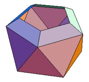
Problem 1: Lighting

Take an icosahedron to get an impression of the problem of lighting "backward" faces of polygons and surfaces with LiveGraphics3D.When you have loaded the package Graphics`Polyhedra` you get an image of an icosahedron with the following expression:

gr1 = Show[ Polyhedron[ Icosahedron ], Boxed -> False ];

WriteLiveForm of LiveGraphics3D will produce the HTML-file. But you will see "shadows" on the backward faces.

WriteLiveForm[ "klafu1.m", gr1 ];

Now you can look at the result.

You may think that the wrong colors of the backward faces of the icosahedron may be due to the closed surface. But you get the same phenomenon with surfaces like the hyperbolic paraboloid with the simple equation  z = x y .

gr2 = Plot3D[ x y, {x,-2,2},{y,-2,2}, Axes -> None, PlotPoints -> 7 ];

WriteLiveForm[ "klafu2.m", gr2 ];

Now the LiveGraphics3D-version.

Problem 2: Clipping

There are several possibilities in Mathematica to restrict values of functions or parts of the domain of definition, e.g. in the image gr2:

a=1.5; gr3 = Plot3D[ xy, {x,-2,2}, {y,-2,2}, PlotPoints->7, PlotRange->{-a,a} ];

A little change and a restriction of the plot domain produce a more agreeable image:

Plot3D[ xy,{x,-2,2},{y,-2,2}, PlotPoints->7, PlotRange->{{-a,a},{-a,a},{-a,a}}];

Axes -> None will suppress the ticks at the box. They are not needed for the transformation with LiveGraphics3D .

gr4 = Plot3D[ x y, {x,-2,2}, {y,-2,2}, PlotPoints -> 7, Axes -> None,

              PlotRange -> {{-a,a}, {-a,a}, {-a,a}} ];

WriteLiveForm[ "klafu3.m", gr3 ]; WriteLiveForm[ "klafu4.m", gr4 ];

In every case LiveGraphics3D does not produce the desired result: klafu3.html ,  klafu4.html

I think that the following Mathematica figure will be adequate:

gr5 = Show[ Graphics3D[ gr2 ], PlotRange -> {-a,a} ];

Also transforming this figure with LiveGraphics3D gives not the desired result:

WriteLiveForm[ "klafu5.m", gr5 ];

klafu5.html

3 Solutions to problems

A solution of problem 1 : Lighting

To switch on some "additional lights" gives an obvious solution. You will find some information about the option LightSources in the Mathematica Help-Browser. This option will be used in the next expressions. More information can be found in Smith and Blachman (1995), p. 254, Wickham-Jones (1994), p. 213 and Schaper (1994), p. 189.

You can get information on the default LightSources:

Options[ Plot3D, LightSources ]

{LightSources -> {{{1.,0.,1.}, RGBColor[1,0,0]},

{{1.,1.,1.}, RGBColor[0,1,0]},

                  {{0.,1.,1.}, RGBColor[0,0,1]}}}

LightSources -> {direction, color} produces parallel light with the direction  direction and with the color color.

Now additional lightsources are used:

lights = {{{ 1, 0, 1}, Red}, {{ 1, 1, 1}, Green}, {{0, 1, 1}, Blue} ,

          (* additional: *)

          {{-1, 0,-1}, Red}, {{-1,-1,-1}, Green}, {{0,-1,-1}, Blue} };

SetOptions[ Plot3D, LightSources -> lights ];

As above the hyperbolic paraboloid and the icosahedron are used to give some explanations.

gr6 = Plot3D[ xy, {x,-2,2}, {y,-2,2}, Axes->None, Boxed->True, PlotPoints->7 ];

Using an adequate choice of ViewPoint you can look at the surface from "below".

Show[ gr6, ViewPoint -> {-2,0,-3} ];

WriteLiveForm[ "klafu6.m", gr6 ];

Here you can look at the HTML-version. And all polygons are colored!

The icosahedron will be treated in an analogous manner :

gr7 = Show[ Polyhedron[ Icosahedron ], LightSources -> lights, Boxed -> False ];

WriteLiveForm[ "klafu7.m", gr7 ];

You can see the positive effect . Compare this example with the old one .

A solution of problem 2 : Clipping

Again we will begin with the hyperbolic paraboloid. The image gr3 is reproduced as gr8a :

gr8a = Graphics3D[ Plot3D[x y, {x,-2,2}, {y,-2,2}, Axes -> True, PlotPoints -> 7,PlotRange -> {-a,a}] ];

Now the surface is clipped by Clip3D from the package

ExtendGraphics`Geometry3D` of  Tom Wickham-Jones:

gr8b = Fold[ Clip3D[#1,#2]&, gr8a, {Plane[{0,0,a}, {0,0,-1}], Plane[{0,0,-a},{0,0,1}]}];  

gr8c = Show[ gr8b, Axes -> True ];

The option Axes will get the value None:

gr8 = Show[ gr8c, Axes -> None ]; WriteLiveForm[ "klafu8.m", gr8 ];

As you can see LiveGraphics3D and the clipping work together. Since above the option LightSources of  Plot3D has been changed also the backward faces are colored. You get the same effect with the icosahedron. Now different colors for the lightsourses are chosen.

gr9 = Show[ Polyhedron[ Icosahedron ], LightSources -> {{{1,0,1}, Red}, {{1,1,1}, Green}, {{0,1,1}, Blue},

{{-1,0,-1}, Tomato}, {{0,-1,-1}, SkyBlueDeep}, {{-1,-1,-1}, GreenDark} }, Boxed -> False ];

a = 3/4; gr10 = Fold[ Clip3D[#1,#2]&, gr9, {Plane[{0,0,a},{0,0,-1}], Plane[{0,0,-a},{0,0,1}]} ];

Show[ gr10 ];

WriteLiveForm[ "klafu10.m", gr10 ];

Here you get the www images .

4 Applications

Klein Bottle

At the beginning three different forms of the Klein bottle are clipped. In Wolfram (1999) you will find the first form on page 995 resp. in the Help Browser at Light_Source_Varations.  Schaper (1994, 257ff.) gives parametrisations of the first and second form. You can get the parametrisations of the second and third form in from this page. If you go to "Klein Bottle Formula" in the Help Browser of Mathematica gives supplementary information on the second form. Also see (Gray, 1998, p. 327).

The parametrisation of the second form can be found in Dieudonné (1972, p. 192, resp. S. 194 of the German translation). See also: The Mathematica Journal, 1, (3), 1991, p. 65.

First form:

bx = 6 Cos[u] (1 + Sin[u]); by = 16 Sin[u]; rad = 4 - 2 Cos[u];

X = If[ Pi < u <= 2 Pi, bx + rad Cos[v + Pi], bx + rad Cos[u] Cos[v]];

Y = If[ Pi < u <= 2 Pi, by, by + rad Sin[u] Cos[v]];

Z = rad Sin[v];

SetOptions[ ParametricPlot3D, LightSources -> lights ];

gr11 = ParametricPlot3D[{X,Y,Z}, {u,0,2 Pi}, {v,0,2 Pi}, PlotPoints -> {48,12}, Axes -> False,

       Boxed -> False, ViewPoint -> {0,-2,-2}];

WriteLiveForm[ "klafu11.m", gr11 ];

klafu11.html

If v is in [0, Pi]  you get this "insight":

gr12 = ParametricPlot3D[ {X,Y,Z},{u,0,2Pi},{v,0,Pi},

PlotPoints -> {48,12}, Axes -> False, Boxed -> False,

ViewPoint -> {0,-2,-2}];

WriteLiveForm[  "klafu12.m", gr12 ];

klafu12.html

Now another clipping:

gr13 = Fold[ Clip3D[#1,#2]&, gr11, {Plane[{0,-10,-1},{4,0,-1}]}];

Show[ gr13, ViewPoint -> {-1.5,0,0} ];

WriteLiveForm[ "klafu13.m", gr13 ];

klafu13.html

Second form:

X = (2 + Cos[u/2] Sin[v] - Sin[u/2] Sin[2v]) Cos[u];

Y = (2 + Cos[u/2] Sin[v] - Sin[u/2] Sin[2v]) Sin[u];

Z = Sin[u/2] Sin[v] + Cos[u/2] Sin[2v];

gr14 = ParametricPlot3D[ {X,Y,Z},{u,0,2 Pi},{v,0,2 Pi},

PlotPoints -> 51, Boxed -> False, Axes -> None ];

WriteLiveForm[ "klafu14.m", gr14 ];

klafu14.html

Now the clipping with two planes:

gr15a = Fold[ Clip3D[#1,#2]&, gr14,

        {Plane[{0.5,0,0.4}, {-0.5,0.25,-1}], Plane[{0,00.8}, { 0, 0,-1}]}];

gr15  = Show[ gr15a ];

WriteLiveForm[ "klafu15.m", gr15 ];

klafu15.html

Third form:

A polynomial representation of the Klein bottle due to Ian Stewart can be found on this web page . "The equation looks odd":

(x^2+y^2+z^2+2*y-1)*((x^2+y^2+z^2-2*y-1)^2-8*z^2)+16*x*z*(x^2+y^2+z^2-2*y-1)==0

You can get the following part of the Klein bottle  with the package ImplicitPlot3D and the following Mathematica expression.

A t t e n t i o n   p l e a s e : The computation needs a lot of time!

(* h = 7; p = 51;

gr16 = ImplicitPlot3D[

(x^2+y^2+z^2+2*y-1)*((x^2+y^2+z^2-2*y-1)^2-8*z^2)+16*x*z*(x^2+y^2+z^2-2*y-1) == 0,

{x,-2,h},{y,-2,h}, {z,-2,h}, PlotPoints -> {p,p,p},

ViewPoint -> {-3,0,1}, Boxed -> False, LightSources -> lights] ;

*)

(* WriteLiveForm[ "klafu16.m", gr16 ]; *)

klafu16.html

(* gr17 = Fold[ Clip3D[#1,#2]&, gr16, {Plane[{-1,-1.5,3}, {3,-2,-2}]}];

   gr18 = Show[ gr17 , Boxed -> False ];

*)

(* WriteLiveForm[ "klafu18.m", gr18 ]; *)

klafu18.html

Fermat

At MathSource there is a notebook of Andrew J. Hanson: FermatSolution.nb . "Solution of Fermat's Equation xⁿ + yⁿ = 1. The notebook shows a projection from four-dimensional space of the so-called projective variety that represents all possible solutions of the equation xⁿ + yⁿ = zⁿ for varying n. What Fermat's Last Theorem states is that none of these solutions can correspond to integer values of x, y and z." Look also at the figures on page 39 of the second edition of the Mathematica-Book. Having done some calculations not incoorperated in this notebook, it is possible to work with the following expressions:

(* gr19 = Show[ Graphics3D[ Table[surface[k1, k2], {k1,1,n}, {k2,1,n}]],

 Boxed -> False, LightSources -> lights ];

*)

(* WriteLiveForm["klafu19.m", gr19]; *)

klafu19.html

You will get more "insight" after clipping:

(* a = 0.2;

   gr20 = Fold[ Clip3D[#1,#2]&, gr19, {Plane[{a,a,a}, {-1,1,-1}] }];  

   gr21 = Show[ gr20, PlotRange -> All ];

*)

(* WriteLiveForm[ "klafu21.m", gr21 ]; *)

klafu21.html

5 Outlook

Some years ago I explored the following surface. At the first glance it seems to be boaring. But there are "inner values" which can be seen when the graphic is rendered or after an adequate clipping. The changed options of lightsources are used.

SetOptions[ Graphics3D, Boxed->False ];

gr22a = ParametricPlot3D[{u Cos[v] Sin[u], u Cos[u] Cos[v],-u Sin[v] },

{u, 0, 3Pi, Pi/18}, {v, 0, 2Pi, Pi/18}, Boxed -> False, Axes -> False ];

Remembering abraded shells on the shore I took the following choice of PlotRange:

gr22b = Show[ gr22a, PlotRange -> {All,{-0.5,10},All} ];

gr22c = Fold[ Clip3D[#1,#2]&, gr22a,{Plane[{0,-0.7,0.5}, {-0.2,1,-1.5}], Plane[{0,-0.5, 0}, { 0,1, 0}]  }];

gr22 = Show[ gr22c ];

WriteLiveForm[ "klafu22.m", gr22 ];

klafu22.html

I think that Michael Trott is the author of the following Mathematica-Oneliner. SetOptions[ Graphics3D, Boxed -> False ] is needed:

gr23a = With[ {stelldode = Stellate@Delete[Dodecahedron[1.6]}

               Show@ Graphics3D@{EdgeForm@Thickness@0.001,

               Stellate[OpenTruncate@Geodesate[stellDode, 3,{0,0,0},1.6], 1.05],

               Stellate@OpenTruncate@Geodesate[stellDode, 3]}];

Clipping and lighting is applied to this object:

gr23b = Fold[ Clip3D[#1,#2]&,gr23a,

            {Plane[{0,0.15,0}, {0,-1, 0}], Plane[{0,-0.15,0}, {0,1,0}]}];

gr23 = Show[ gr23b, Boxed->False,PlotRange->All, ViewPoint->{0,-3,0},LightSources->lights ];

WriteLiveForm[ "klafu23.m", gr23 ];

klafu23.html

Now the hole is filled:

Needs[ "Graphics`Shapes`" ]; gr24a = Graphics3D[ Sphere[0.98,32,16] ];

Show[ gr24a ];

There is a remark on "placing several lightsources at the same point" in Smith and Blachman (1995, p.260). That will produce "more intense illumination".

gr25 = Show[ {gr23,gr24a}, Boxed -> False,

ViewPoint -> {0,-3,0}, LightSources ->

 {{{1,0,1}, Gold}, {{0,1,1}, Gold}, {{1,1,1}, Yellow},

 {{1,1,1}, Red},{{1,0,1}, Gold}, {{0,1,1}, Gold}, {{1,1,1}, Gold},

 {{-1, 0,-1}, Yellow}, {{ 0,-1,-1}, Yellow},

{{-1,-1,-1}, Yellow}, {{-1,-1,-1}, Red}}];

WriteLiveForm[ "klafu25.m", gr25 ];

klafu25.html

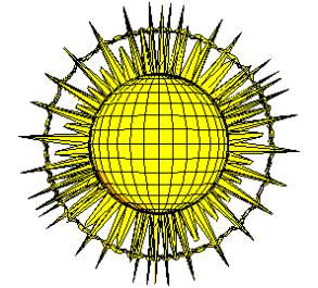
Let the sun shine bright over the conferences at Klagenfurt. Click here for the homepage of the author: Ralf Schaper

References

Jean Dieudonné (1972) Treatise on Analysis, volume III. Academic Press, New York: (In German: (1976) Grundzüge der modernen Analysis, Band 3. Vieweg, Braunschweig).

Alfred Gray (1998) Modern Differential Geometry of Curves and Surfaces with Mathematica. CRC Press, Boca Raton.

Schaper, R. (1994) Grafik mit Mathematica Bonn: Addison-Wesley.

Smith, C. and Blachman, N. (1995) The Mathematica Graphics Guidebook. A. Wesley, Reading.

Wickham-Jones, T. (1994) Mathematica Graphics. Springer, Reading.

Wolfram, S. (1991) The Mathematica Book, 2nd ed. Addison-Wesley, Redwood City.

Wolfram, S. (1999) The Mathematica Book, 4th ed. Wolfram Media, Champaign.

URLs

Fermat ImplicitPlot3D Klein Bottle

LiveGraphics3D

HomePage Documentation Examples Two Surfaces Polyhedra Interactive Uniform Polyhedra

Hints for the Installation

You have to set the right path in the package LiveGraphics3D` to save the HTML-files.In his book Tom Wickham-Jones describes a Mathematica-package for additional clipping routines of 3D-graphics. You can get the packages on MathSource with this URL:http://www.mathsource.com/Content/Enhancements/Graphics/3D/0208-976 . Our notebook needs only the packages

Geometry.m, Geometry3D.m, NonConvexTriangulate.m and SimpleHull.m .

Work will be more easy if the mentioned files are loaded in a directory also named ExtendGraphics in the directory Autoload in AddOns:

E.g.:  Mathematica/4.1/AddOns/Autoload/ExtendGraphics.

You can find the following example in the book of Wickham-Jones ( p. 440 ). You may proceed in the following manner after loading the mentioned packages:

Needs[ "ExtendGraphics`Geometry3D`" ]

surf = Graphics3D[ Plot3D[Sin[x y], {x,-Pi,Pi}, {y,-Pi,Pi}, PlotPoints- > 30 ]];

?Plane

Plane[ c, n] represents the plane line which passes through c and is normal to n

gr26a = Fold[ Clip3D[#1,#2]&, surf, {Plane[{0,0,0.5},{0,0,-1}], Plane[{0,0,-0.5}, {0,0,1}]}];

Show[ gr26a ];

End of the citation.

gr26 = Show[ gr26a, Boxed->False, Axes->None, DisplayFunction->Identity ];

WriteLiveForm[ "klafu26.m", gr26 ];

klafu26.html

At last a variation with a "sloping" plane:

gr27a = Fold[ Clip3D[#1,#2]&, surf, {Plane[{Pi/2,0,0}, {-1,1,-1}]}];

gr27 = Show[ gr27a, Boxed -> False, Axes -> None ];

WriteLiveForm[ "klafu27.m", gr27 ];

klafu27.html

Fig. 1	Fig. 2: Let the sun shine bright over the conferences at Klagenfurt

Goto
	Begin of article		Contributions by authors
	Begin of session		Main page

Mittels Computer zu mathematischen Entdeckungen

Grosio Stanilov and Lidia Stanilova

Sofia, Bulgaria

Wir demonstrieren an einigen Beispielen, welch wichtige Rolle die Computergraphik spielen kann, um auf neue wissenschaftliche Probleme zu kommen. Dabei es handelt sich um Untersuchungen, die auch von Schülern und Lehrern umgesetzt werden können.

Betrachten wir ein Einheitsquadrat OABC mit Koordinaten O(0,0), A(1,0), B(1,1), C(0,1) und eine bewegliche Gerade g = MN mit M(m,0) und N(0,n). Wir wollen alle Geradenschnitte von g mit OABC untersuchen.

Für g Ç AB = P und g Ç BC = Q bestätigt man leicht

		(1)

Satz 1.

(i) Wenn m Î (0,1) ist, dann gilt:

Ist {	a)		dann ist der Schnitt {	MQ
	b)			MP
	c)			MN
	d)			MQ

(ii) Wenn m ³ 1 ist, dann gilt:

Ist {	a)		dann ist der Schnitt {	PN
	b)			PQ

(iii) Wenn m < 0 ist, dann gilt:

Ist {	a)		dann ist der Schnitt {	PN
	b)			QN

In allen anderen Fällen gibt es keine Quadratschnitte.

Durch die Gleichungen (1) sind für die entsprechenden Fälle diverse Flächen bestimmt, z. B.

PQ^2 (m, n) =			m³1,
PN^2 (m, n) =		{	m³1,
			und m<0,

Diese Flächen schneiden sich längs der Kurve

PC^2 (m, n=1) =

m ³1

Satz 2.

Das bedeutet, die Länge des Schnittes ist auch eine stetige Funktion in den Ecken des Quadrats; Fig. 1 zeigt beide Flächen und auch deren Schnittkurve.

Fig. 1	Fig. 2

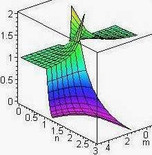
Beiden Figuren ist etwas Besonderes zu entnehmen: Die beiden Flächen schneiden sich nicht "glatt", denn es gilt:

Satz 3. Die Länge der Quadratschnitte (m-fest) ist für jedes n eine stetige, aber nicht differenzierbare Funktion in den Quadratecken.

Dieses Ergebnis ist zu vergleichen mit dem entsprechenden Ergebnis für Würfelschnitten. Stanilov und Stanilova (1999) und Stanilov e.a. (2001) beweisen:

Satz 4. Die Flächeninhaltsfunktion bei den Würfelschnitten ist eine stetige und auch differenzierbare (genauer 1-mal differenzierbare) Funktion in den Würfelecken.

Man kommt von hier in natürlicher Weise zu neuen wissenschaftlichen Problemen: Wie lassen sich die Sätze 3 und 4 auf den 4-dimensionalen Raum oder sogar auf einen Raum beliebiger Dimension verallgemeinern? Welche Beziehung besteht zwischen der Dimension des Raumes und der Differenzierbarkeit des Schnittes?

Vermutung. Es gilt die Beziehung r = n – 2, wobei n die Dimension des Raumes und r die Ordnung der Differenzierbarkeit des Schnittes in den Ecken des Hyperwürfels bezeichnet.

Ich erinnere an ein Ergebnis von Stanilov (2000). Es seien ABCDA₁B₁C₁D₁ ein Einheitswürfel und e = MNK die Schnittebene, die durch die Gleichungen bestimmt ist:

Bei festem m und n hängt der Schnitt von k ab. Man erhält folgenden Teilungspunkt:

(2)

Durch diese Gleichung wird eine “exotische” Fläche definiert. (2) ist “fast äquivalent” zu

(3)

oder zu der Gleichung

mnk = mn + nk + km

(4)

Mit Maple 6 läßt sich die Fläche (4) leicht zeichnen (Fig.2).

Weiters, wenn man die rechte Seite von (2) mit f(m, n) bezeichnet und (3) benutzt, sieht man, dass die Funktion der folgenden Funktionalgleichung

k = f ( f ( m, k), f (n, k) )

(5)

genügt. Gleichung (5) hat großes Interesse gefunden, Benz e.a. beweisen:

Тheorem 1. Es sei G eine nichtleere offene Menge von R und D : = G´G. Es gibt genau 2^À verschiedene Lösungen f : D ® R, welche der Gleichung (5) genügen.

Ersetzt man (5) durch

m = f (n, f (m, n) ), n = f ( m, f (n, m) )

(6)

So kann man beweisen:

Proposition 1. Alle multiplikativen Lösungen von (6) sind:

f (m, n) = c/xy ( c=const)

(7)

Theorem 2. Es existiert genau eine harmonische Lösung von (5), nämlich die rechte Seite von (2).

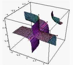
Wenn wir die Fläche (4) mit Ebenen orthogonal zu der Achse Oz schneiden, bekommen wir Hyperbeln (Fig. 3). Daraus folgt:

Satz. Die Fläche (4) ist geometrischer Ort von orthogonalen Hyperbeln, welche die Achse Oz schneiden und welche in Ebenen liegen, die orthogonal zu Oz sind, so dass die Mittelpunkte von diesen Hyperbeln eine weitere Hyperbel H bilden, welche

a) in der Ebene Ox z liegt (x die Winkelhalbierende der Achsen Ox, Oy),b) O enthält,c) den Mittelpunkt E(1,1,1) hat.

Wenn man “orthogonale Hyperbeln” durch Kreislinien ersetzt, erhält man folgende bemerkenswerte Fläche (Fig. 4):

z [ (x-1)^2 + (y-1)^2 –2 ] = x^2 + y^2

(8)

Fig. 3	Fig. 4

Man erhält drei neue Familien von Flächen, wenn man in (3) die Variablen x, y, z (an Stelle von m, n, k) durch beliebige Funktionen ersetzt:

I
II
III

Jede solche Fläche erzeugt eine entsprechende Funktionalgleichung, auf welche die Ergebnisse für Gleichung (5) anwendbar sind.

Nun betrachten wir einige Beispiele.

Fig. 5: Ersetzt man orthogonale Hyperbeln durch Parabeln, Mittelpunkt mit Brennpunkt analog Fig. 4:  z(y^2 – 2 x) =10	Fig. 6: Zu Familie II gehört die Fläche exp(x)+exp(y)+exp(z) = exp(x) exp(y) exp(z)

Fig. 7: Zu Familie II gehört die Fläche	Fig. 8: Zu Familie I gehört die Fläche sin(x)sin(y)+sin(y)sin(z)+sin(z)sin(x)= sin(x)sin(y)sin(z)

Zum Schluß zeigen wir noch drei Flächen, die besonders attraktiv sind (Fig. 9-11)

Fig. 9: Fläche   z = (x^2 y^2 +x^2 + y^2)^7—durch eine passende Ebene geschnitten	Fig. 10: Fläche   sin z = x y

Die s.g. Versiera von Maria Agnesi wird durch folgende Gleichung bestimmt

y = 8 r³ /(4r² + x²),

wobei r der Radius des Kreises und x beliebig ist. Dann betrachten wir die Fläche

z = 8y³ /(4y² + x²)

für beliebige x und y (Fig. 7 und 8). Die Ebene y=const ergibt eine Versiera. Durch z = const. bekommt man eine interessante Animation und neue ebene Kurven.

Fig. 11a	Fig. 11b

References

Stanilov, G., Stanilova, L. (1999) Neue Max Bill Würfelschnitte und deren Anwendung in der bildenden Kunst. Beiträge zum Mathematikunterricht, Franzbecker, Hildesheim, 501-506.

Stanilov, G. , Boychev, P. and Cankov, J. (2001) Mittels Computer zur mathematischen Entdeckungen. Beiträge zum Mathematikunterricht 2001, Franzbecker, Hildesheim.

Stanilov, G. (2000) Cubic sections by moving plane and application in the finite art. Proc. Intern. Congress “Constantin Caratheodory in his origin. Hadronic Press, Vissa-Orestiada, Greece.

Benz, W., Samaga, H.-J. and Stanilov, G. (2001): Stanilov,s Functional Equation is exorbitant (Submitted for publication).

http://www.fmi.uni-sofia.bg/fmi/geometry/stanilov

Goto
	Begin of article		Contributions by authors
	Begin of session		Main page

Cubic section by moving plane

Yulian Tsankov

Sofia, Bulgaria

1. The problem

2. Using Mathematica, we give a program

3. Here is the source of our program

In this paper we study the section and its area function of a cube with a moving plane. Stanilov and Stanilova (1999) and Stanilov e.a. (2001) give a usual vector method for this purpose. We give another coordinate method and a program for numerical investigations. For the Stanilov method it is necessary to determine the area function and one must consider many different cases. Our method leads to a universal program without restrictions.

1 The problem

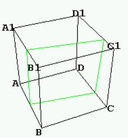
We consider the unit cube. The moving plane e (M N K) is determined by the points M, N, K, where

The moving plane cuts the edge-straight-lines of the cube in points:

e Ç AA1 = S,	e Ç CC1 = W,	e Ç DD1 = Y,
e Ç AD = T,	e Ç CD = V,	e Ç B1C1 = X,
e Ç B1A1 = U,	e Ç C1D1 = P,	e Ç A1D1 = Z.

Notation

Theorem 1. Let m < 0 and n < 0.

	If	the cubic section is	with area functions
1.	kÎ(0, k0)	KWYS
2.	kÎ(k0 , m0)	KWPZS
3.	kÎ(m0 , n0)	KWPU
4.	kÎ(n0, 1)	KXU
5.	k Ï (0 , 1)		there is no cubic section.

-¥		0		k0		m0		n0		1		+¥
	0		4		5		4		3		0

Table 1

The number of the peaks (when m < 0 and n < 0) of the section in the different intervals is shown in Table 1. Thus the area function is given as a partial smooth function. One can prove (Stanilov and Stanilova 1999, Stanilov e.a. 2001):

Theorem 2 The area function is exactly 1- differentiable in the dividing points, i.e. in the vertices of the cube.

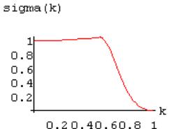
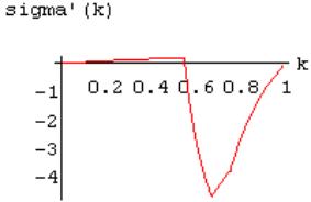
Fig. 1 shows the graph of the area function in the case m = - 2, n = -3. Fig. 2 shows the graph of the derivative of the area function. Both figures illustrate the validity of Theorem 2.

Fig. 1	Fig. 2

We introduce a coordinate system as follows:

0ºB(0,0,0),

A(0,1,0),

C(1,0,0),

B1(0,0,1)

Then

2 Using Mathematica, we give a program

For the cubic section and its area - function for given m, n, k Î(-¥, ¥).

Then if we fix any two of these parameters we can animate the cubic sections and together its area functions.

If we fix one of these parameters then the area function determines a surface, which can be visualized.

The programming code to visualize the cubic planes, may be written in any language, containing Boolean and loop operators. Besides these operators, Mathematica has many built-in functions for graphics and list processing which facilitate the realization. Thus, in using Mathematica, graphic batches are not necessary to be loaded as it is in using for instance Pascal, C, or C++.

Here the sequence follows: First of all, it is checked which of the twelve intersections and the three coordinates are in the interval [0, 1] as the parameters are constant. These points are the picks of the plane of the cube with the plane e.

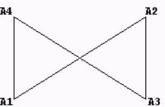
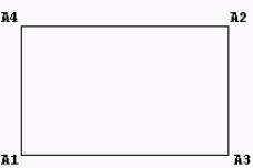
To plot the poliangle, in which the plane intersects the cube, we connect its picks using the command line of Mathematica. If, however, the points are not arranged we might not get a protuberant poliangle. For example, if we consider the points A₁(0,0), A₂(1,1), A₃(1,0), A₄(0,1), and connect them in the given order, we get Fig. 3. These are the commands in Mathematica:

Show[Graphics[Line[{{0,0},{1,1},{1,0},{0,1},{0,0}}]],

Graphics[Text[ FontForm["A1",{"Courier-Bold",12}],{-0.05,-0.05}]],

Graphics[Text[ FontForm["A3",{"Courier-Bold",12}],{1.07,-0.05}]],

Graphics[Text[ FontForm["A2",{"Courier-Bold",12}],{1.05,1.05}]],

Graphics[Text[ FontForm["A4",{"Courier-Bold",12}],{-0.05,1.05}]]]

The same points may be connected in a way to get a protuberant poliangle as it is shown in Fig. 4.

Fig. 3	Fig. 4

In order to avoid errors we sort the point in such a way that allows us to get a protuberant poliangle after connecting them.

Here the sequence follows which sorts through up to n points A₁, A₂,…, A_n (the points are given with their coordinates in a standardized coordinate system with a point O beginning). We first determine the coordinates of the point C through the formula:

Then consider the vectors

The end points of these vectors lie on a circle with radius of length 1. We arrange these vectors by the size of their angle with the Ox axis. Without finding the angle, this might be achieved in the following way: First we choose the vectors whose second coordinate (y) is positive and sort them by decreasing first (x) coordinates, or if their second coordinate is smaller or equal to zero we sort them by going up the first coordinate (Fig. 5) .

Fig. 5

We find the area of a poliangle in the following way: The poliangle is divided to triangles. The triangles do not intersect each other and do not have joint sides. This kind of division is named triangulation (Fig. 6).

Fig. 6

We find the areas of all these triangles (the formula of the coordinate aspect vector product is convenient in a computer calculation) and sum them. Using this sequence we can see how the area of the section looks and to figure out the area. We can also calculate the area in a very thick web of values for the m, n, and k parameters and find the maximal one. This can assist us in finding the minimal and maximal values of the area function.

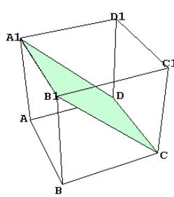
Example 1. If m = 0.5, n = 3, k = 5, the section is shown in Fig. 7 and the area is 1.01871

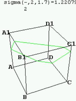
Example 2. If m = 3/2, n = 1, k = 1.7, the section is shown in Fig. 8 and the area is 1.22076

Fig. 7: sigma(0.5,3,5) = 1.01871	Fig. 8: sigma(3/2,2,1.7) = 1.22079
Fig. 9: sigma(200,1,1) = 1.41069	Fig. 10

Example 3. The section with maximal area (which is obtained in comparing the segment areas in a very thick web of values for m, n, and k) is shown in Fig. 9 for m = 200, n = 1, k = 1, the area is approximately Ö2.

If we fix one of the parameters m, n, k we get a surface. Namely the surface of the area functions of all sections for such parameters. From a geometrical point of view, those surfaces are interesting, for which the planes cut some vertex of the cube.

Example 4. If k = 1, we look for all sections which cut the cube in the vertex B₁, m, n-arbitrary. Fig. 10 illustrates the surface of all area functions when k = 1, m Î (0.1, 3), n Î (0.1, 3).

3 Here is the source of our program

================================================================================

NN[n_,m_,k_]={n,0,0};

M[n_,m_,k_]={0,m,0};

K[n_,m_,k_]={0,0,k};

S[n_,m_,k_]={0,1,k*(m-1)/m};

W[n_,m_,k_]={1,0,k*(n-1)/n};

Y[n_,m_,k_]={1,1,k*(n*m-n-m)/(n*m)};

T[n_,m_,k_]={n*(m-1)/m,1,0};

V[n_,m_,k_]={1,m*(n-1)/n,0};

X[n_,m_,k_]={n*(k-1)/k,0,1};

U[n_,m_,k_]={0,m*(k-1)/k,1};

P[n_,m_,k_]={1,m*(n*k-n-k)/(n*k),1};

Z[n_,m_,k_]={n*(m*k-k-m)/(m*k),1,1};

LP[n_,m_,k_]=N[{NN[n,m,k],M[n,m,k],K[n,m,k], S[n,m,k], W[n,m,k],Y[n,m,k],

T[n,m,k],V[n,m,k],X[n,m,k], U[n,m,k], P[n,m,k],Z[n,m,k]} ];

cub={Graphics3D[Line[{{0,0,0},{1,0,0},{1,1,0},{0,1,0},{0,0,0}}],

PlotRange->All, Boxed->False],

Graphics3D[Line[{{0,0,1},{1,0,1},{1,1,1},{0,1,1},{0,0,1}}]],

Graphics3D[Line[{{0,0,0},{0,0,1}}]],

Graphics3D[Line[{{1,0,0},{1,0,1}}]],

Graphics3D[Line[{{1,0,0},{1,0,1}}]],

Graphics3D[Line[{{1,1,0},{1,1,1}}]],

Graphics3D[Line[{{0,1,0},{0,1,1}}]],

Graphics3D[Text[ FontForm["B",{"Courier-Bold",12}], {-0.05,-0.05,0}]],

Graphics3D[Text[ FontForm["A",{"Courier-Bold",12}], {-0.05,1.05,0}]],

Graphics3D[Text[ FontForm["C",{"Courier-Bold",12}], {1.05,-0.05,0}]],

Graphics3D[Text[ FontForm["D",{"Courier-Bold",12}], {1.1,1,0}]],

Graphics3D[Text[ FontForm["B1",{"Courier-Bold",12}], {-0.05,-0.05,1.05}]],

Graphics3D[Text[ FontForm["A1",{"Courier-Bold",12}], {-0.05,1.05,1}]],

Graphics3D[Text[ FontForm["C1",{"Courier-Bold",12}], {1.05,0.05,1}]],

Graphics3D[Text[ FontForm["D1",{"Courier-Bold",12}], {1.05,1.05,1}]]};

Show[cub,ViewPoint->{-1.444, -2.316, 2.000}];

Test[P_]:=If[P[[1]]>=0 && P[[1]]<=1 && P[[2]]>=0 && P[[2]]<=1 &&

P[[3]]>=0 && P[[3]]<=1, True,False]

pl[a_,b_,c_]:=DeleteCases[

Table[

If[Test[LP[a,b,c][[i]]],LP[a,b,c][[i]],Null],

{i,1,12}],

Null]

sss[l_]:= Module[{u}, If[l != {}, sss1[l], l]]

sss1[b_]:= Module[{ls, sls, ymaxx, l1, k, p, l2},

Cent = Sum[b[[i]], {i, Length[b]}]/Length[b];

vectori = Table[Cent - b[[i]], {i, Length[b]}];

t2t = Table[{vectori[[i]][[1]]/

Sqrt[(vectori[[i]][[1]])^2 +(vectori[[i]][[2]])^2],

vectori[[i]][[2]]/

Sqrt[(vectori[[i]][[1]])^2 +(vectori[[i]][[2]])^2]},

{i, Length[b]}];

t3t = Table[Join[{t2t[[i]]}, {i}], {i, Length[b]}];

s1=1;

s2=1;

Table[

Which[

t3t[[i]][[1]][[2]]>= 0, arr1[s1] = t3t[[i]]; s1++,

t3t[[i]][[1]][[2]]< 0, arr2[s2] = t3t[[i]]; s2++],

{i, 1, Length[t3t]}];

ppp = Join[Reverse[Sort[N[Table[arr1[i], {i, s1 - 1}]]]],

Sort[N[Table[arr2[i], {i, s2 - 1}]]]];

ListForPlot1 = Table[b[[ppp[[i]][[2]]]], {i, Length[b]}];

ListForPlot = Join[ListForPlot1, {ListForPlot1[[1]]}];

ListForPlot]

ttt[po_]:=Module[{u}, leng[ve_]:= Sqrt[ ve.ve ];

vec[v1_,v2_]:={v1[[2]]*v2[[3]]- v2[[2]]*v1[[3]],

-v1[[1]]*v2[[3]]+ v2[[1]]*v1[[3]],

v1[[1]]*v2[[2]]- v2[[1]]*v1[[2]]};

plosh[t1_,t2_,t3_]:=(1/2)*leng[vec[t1 - t2, t3 - t2]];

area = 0;

For[i=1, i <= Length[po]-2,i++,

area=area+plosh[po[[1]],po[[i+1]], po[[i+2]]]

];

area]

================================================================================

References

Stanilov, G., Stanilova, L. (1999) Neue Max Bill Würfelschnitte und deren Anwendung in der bildenden Kunst. Beiträge zum Mathematikunterricht, Franzbecker, Hildesheim, 501-506.

Stanilov, G. , Boychev, P. and Cankov, J. (2001) Mittels Computer zur mathematischen Entdeckungen. Beiträge zum Mathematikunterricht 2001, Franzbecker, Hildesheim.

http://www.fmi.uni-sofia.bg/fmi/geometry/yulian/

Goto
	Begin of article		Contributions by authors
	Begin of session		Main page

[1] Further partners in the project were Center for Open and Distance Learning of the Johannes Kepler University, Linz, Ars Electronica Center, Linz, UNI SOFTWARE PLUS, Hagenberg and Wolfram Research Europe, Oxfordshire.

[2] The didactic framework has been developed in the project IMMENSE (Interactive Multimedia Mathematics Education in Networked universities for Social and Economic sciences) of a consortium led by the Johannes Kepler University Linz and the Austrian Ministry of Education, Science and Culture. Further partners were Center for Open and Distance Learning of the University of Linz, Ars Electronica Center, Linz, UNI SOFTWARE PLUS, Hagenberg and Wolfram Research Europe, Oxfordshire.

[3] MeetMATH@Business & Economy is available free; see: www.flll.jku.at/div/meetmath/

[4] More details about categorization of learning objectives can be found in Becker (1991.

[5] For further details on concepts of visualization see e.g. Kadunz (2000), Volkert (1986).