Strand 6:
Mathematical modelling with technology
Jenny Sharp
Plymouth, UK
|
Plenary lecture |
The use of technology in developing mathematical modelling skills |
|
Differential equations instead of analytical methods |
|
|
Laplace Transform and electrical circuits: An interdisciplinary learning tool |
|
|
Mathematical application projects for mechanical engineers — Concept, guidelines and examples |
|
|
Cross curriculum teaching and experimenting in math & science courses using New Technology |
|
|
Mathematical modelling with use of Cabri |
|
|
Modelling human growth |
|
|
Investigating bridges and hanging chains |
|
|
Model of deformations of fluid particles due to electric field |
|
|
Introducing models and modelling through spreadsheets |
|
|
Software Maple in the teaching of ODE’s |
|
|
Discrete delayed population models with Derive |
1. Mathematical modelling with secondary school students
2. Mathematical modelling with upper secondary students
3. Mathematical modelling with university students
4. Plenary session – The use of technology in developing mathematical modelling skills
When asked to chair the strand ‘Modelling with Technology’ I had to write a short paragraph for the Conference web page to describe the strand to potential contributors. It was difficult to describe succinctly what is meant by modelling. If you ask ten mathematicians what is modelling then you will probably get ten different answers. After posing the question to my colleagues here at Plymouth I put together the following descriptor:
Mathematical modelling is the application of mathematics to solve realistic problems. Many teachers are unhappy about working with problems where the answer is not defined, as is often the case when really solving real problems. The students have to know which mathematics to apply and when. How can technology be used in this area of mathematics to make the teacher more confident to tackle an unknown problem with the students?
Issues raised are:
 How confident should the student be with the technology?
Should you use the technology as a 'black box' to concentrate on the
modelling aspects?
Assessment issues when it appears that the technology has 'done' the
mathematics - should we be assessing modelling skills instead?
True 'real' world problems are needed in order for the student to
understand the need to use technology to solve an otherwise unsolvable problem.
This descriptor provided the conference with a wide variety of papers covering the topic ‘Modelling with Technology’. Out of the thirteen papers, the speakers ranged from school teachers, to university professors of mathematics and engineering and also mathematics education. Each paper related the speakers first hand experience of ‘modelling with technology’. Here again the range was diverse; we had papers describing work with students aged 14, with students aged 16 – 18 and with students at University. Each paper described how technology was used; again the technology ranged from hand held technology and data loggers, to spreadsheets, through to Computer Algebra Systems. I am going to attempt in this short overview to summarise the papers in this strand and bring out some important outcomes from the conference. I have decided to organise the papers in this overview in ‘age’ groups; those dealing with students up to the age of 16, those students aged between 16 and 18 and then finally university students.
1 Mathematical modelling with secondary school students
There were three papers which dealt with students up to the age of 16; two by André Heck; ‘Modelling Human Growth’ and ‘A practical Investigation Task with the Computer at Secondary School: Bridges and Hanging Chains’, and part of the paper by Brigitta and Klaus Aspetsberger; ‘Cross Curriculum teaching and Experimenting in Maths and Science Courses Using New Technologies’. Heck’s work was with students who were aged 15-16 years old who had no experience with practical investigation tasks, and who have not previously worked with Coach (the software developed by AMSTEL Institute. The main objectives are to let the pupils work with real data and with diagrams; experience how much useful information can actually be obtained from diagrams; see that the change of a quantity is often as important and interesting as the quantity itself; practice ICT-skills; carry out practical work in which they can apply much of their mathematical knowledge. The topic which the students worked on, Modelling Human Growth, provided a rich environment for the students, it is a topic close to the heart of many students. Heck reported that the students managed well with the technology although, on reflection, more time is needed to allow the students to become familiar with it before having to work on assignments etc. In the question session, a number of the audience suggested that, although the topic of growth was one rich in mathematics and ideal for introducing modelling skills, it was one that they would consider with reservations due to the sensitive nature of young people at this age about their weight.
Heck’s second paper explored a different topic - modelling bridges. Again the software Coach was used to great advantage in being able to record and analyse measurements from digital images of bridges. Again the students seemed to cope well with the technology. However they complained that they were not doing enough maths, that it seemed to be a technology lesson rather than the maths lesson. This is an important point that we must remember when we are introducing technology into the classroom – when are we teaching technology and when are we using technology to teach mathematics. Heck’s work showed that we cannot do both at the same time.
From computers to hand held technology; Brigitta and Klaus Aspetsberger included in their paper ‘Cross Curriculum Teaching and Experimenting in Maths and Science Courses Using New Technologies’ a description of some work done with able 14 year old students using the TI-92 and the CBL. They were trying to provide enrichment activities for the students using the new technology while at the same time trying to provide examples of cross curriculum teaching. Similar to Heck above they encountered problems with introducing the technology and the mathematics at the same time, the students struggled with the technology mainly because the instructions were in English and they were unfamiliar with interpreting the output.
2 Mathematical modelling with upper secondary students
The use of technology in modelling for this age group was demonstrated by Per Broman in his paper ‘Mathematical Modelling with CABRI’ and by Brigitta and Klaus Aspetsberger in ‘Cross Curriculum Teaching and Experimenting in Maths and Science Courses Using New Technologies’. Broman discussed using CABRI in tackling what appeared to be a relatively simple problem. However as he demonstrates, the use of the technology allows the problem to be viewed from many different ways, thus allowing the students a wider range of mathematical concepts to explore. Aspetsberger described their experiment working with students and teachers of mathematics and science. Using the CBL and the TI-92 they ran experiments testing the quality of the water in their region. Overall the experiment was a success in as much as the students were motivated and enjoyed the experience. The technology enabled them to analyse results that were normally beyond them. However the authors found that they had underestimated the amount of time it would take to ensure that the students were familiar with the technology, a point also found in the reports of using technology with the younger children.
3 Mathematical modelling with university students
This section had the majority of papers for this strand. This is not altogether surprising, university curricula are such that technology can be incorporated without the fear of it taking up valuable teaching time as is often the case with a ‘national curriculum, for students aged up to 18. There were several papers, which dealt with mathematics for mathematics students, while some demonstrated how mathematics can be made practical and applicable to students of other disciplines such as engineering and physics.
Duncan Lawson’s paper ‘A Discrete Introduction to Modelling’ detailed the dangers of introducing new mathematics, new technologies and the new techniques of mathematical modelling at the same time. It is important that students are only learning one thing at a time and if it is a course on mathematical modelling they should be using mathematics and technology that they are familiar with. This was the first paper of the conference and these ideas were echoed in many of the following presentations. Mazen Shahin in ‘Modelling with Difference Equations using Derive’ demonstrated the use of Derive when introducing difference equations, with the technology the students were able to explore graphically and numerically rather than algebraically. This allowed them to gain a deeper understanding of the processes rather than being engulfed by the algebra. Pavel Prazak in ‘Software Maple and MATLAB in teaching of ordinary differential equations’ continued this theme; the visualisation that the software provides allows the students to gain a far deeper understanding than when solved algebraically.
The above three speakers related the experiences of mathematics students. The rest of the papers in this strand showed how technology helps when teaching the mathematical content of other disciplines. George Aide and Bogdan Zoltowski (‘Differential Equations in Maths and Physics instead of Analytical Methods’) teach physics at undergraduate level and have found that the curriculum is being driven by the technology and vice versa. The technology allows higher order differential equations to be studied; however this requires that new mathematical concepts are required. Students of electronics were addressed by Albano (Laplace Transform and Electric Circuits; and inter disciplinary learning tool’) and Hristov (Model of deformations of fluid particles to electric fields’). Albano demonstrated how the CAS can be used as a support tool to help the students solve differential equations while Hristov showed that careful selection of problems can lead to a lesson in modelling as opposed to solving the problem; an important point made by many speakers, we need to teach the students the skill of modelling.
As those mathematicians who try to teach mathematics to engineering students know it is often difficult to make the mathematics applicable to the engineering world. Burkhard Alpers in his paper ‘Mathematical Application Projects for Mechanical Engineers – Concept, Guidelines and Example’ demonstrated how he has managed to solve this problem. By putting together ‘projects’ for the students to work on where they must demonstrate all necessary requirements of good mathematical modelling – understanding the problem, formulating the mathematics, solving the mathematics (using technology), analysing the results (often by building an object), he has demonstrated that it is possible. The use of the technology enables the students to tackle real problems, something that is essential in the training of our mechanical engineers.
4 Plenary session – The use of technology in developing mathematical modelling skills
By coincidence the plenary session for this strand was the last presentation in the strand. John Berry was able to draw upon the papers already presented, in this strand and elsewhere in the conference to provide an overview as well as some though provoking comments. He pointed out the dangers of using technology unnecessarily, too often we feel pressured into using the latest computer programme or hardware simply because it is there. Many students already see mathematicians as some sort of magicians; we are in danger of perpetuating this myth if we allow more and more mathematics to be done at the click of a mouse or the press of a button. Technology plays a valuable role in the teaching and learning of mathematics but we should remember that it is the appropriate use that makes it most valuable.
5 Conclusion
This summary of the papers presented at the conference is very brief and obviously one should refer to the original paper for exact details. My thanks go to the speakers of this strand for providing the conference with a varied and interesting range of papers. However a speaker is no good without an audience and it was a pleasure to be chairing an audience, which contributed to the session with valued comments, questions and suggestions. It was often difficult to bring the session to an end when so many discussions were being had. I hope that this conference has been a springboard for those speakers who spoke for their first time as well as the seasoned presenters, a chance to realise that their work in this field is important and that they can make a difference to how mathematics is taught and learnt.
The use of technology in developing
mathematical modelling skills
John Berry
Plymouth, UK
2. Pupils views of mathematics and the work of mathematicians
3. The role of technology in mathematical modelling
4. Students' modelling working styles
1 Introduction
Much has been said about the importance of mathematics in the school and college curriculum and much has been written about what should be included in the curriculum for the beginning of the twenty first century. Often there is a tension between the school curriculum and the perceived needs of college and university mathematicians. Too often the mathematics curriculum at all levels is seen as a ‘body of knowledge’ which needs to be delivered in order to provide an ‘acceptable graduate in mathematics’. In this era of powerful software on hand-held and computer technologies we need to review the procedures and rules that have been the central focus of the mathematics curriculum for over one hundred years. That is not to say that we do not need some of the traditional skills so that students can make effective use of the technology. However there are important generic skills that mathematics provides, and to the employer of our graduates these skills are often more important than the actual mathematics that they have learnt.
Problem solving skills are often the most quoted generic skills that should be developed as part of a mathematics curriculum. The NCTM Principles and Standards for School Mathematics (2000) identifies problem solving as important for all school pupils:
Instructional programs from prekindergarten through grade 12 should enable all students to
build
new mathematical knowledge through problem solving;
solve
problems that arise in mathematics and in other contexts;
apply
and adapt a variety of appropriate strategies to solve problems;
monitor
and reflect on the process of mathematical problem solving.
By learning problem solving in mathematics, students should acquire ways of thinking, habits of persistence and curiosity, and confidence in unfamiliar situations that will serve them well outside the mathematics classroom. In everyday life and in the workplace, being a good problem solver can lead to great advantages. (Emphasis added)
Problem Solving in Mathematics is often thought of in three ways:
pure
mathematics investigation activities,
mathematical
modelling,
mathematics
problems and real problem solving.
Tasks that have been classified as “Mathematics Problems” and “Real Problem Solving” are those examples and exercises that are traditionally found in mathematics textbooks and other classroom resources. They usually provide students with opportunities to practice the procedures, rules and skills of the traditional mathematics curricula. “Mathematical Modelling” and “Mathematical Investigation” tasks often require students to develop their own models and explore their own conjectures in order to meet some criteria. They often provide good opportunities for students to develop problem solving and investigation skills that are useful in all areas of mathematics.
In this paper we focus on mathematical modelling which we view as a process consisting of three main stages. First, a problem in the real world is formulated as a mathematical problem. Second, the mathematical problem is solved. Third, the solution is translated back into the original context and the results interpreted to help solve the original problem. It is important for students to experience all stages of the process. This process can be summarised by the following diagram: the modelling cycle:
|
|
|
|
|||
|
|
Fig. 1: The Mathematical Modelling Cycle |
|
Many courses and textbooks in mathematical modelling do not actually address the process of modelling but focus on teaching examples of mathematical models and the mathematical techniques needed to use these models. This leads to a conflict of learning interests. I would argue that the teaching of modelling skills should be emphasized in a modelling course and that students should only use the mathematics skills that are familiar to them. Standard models and familiar mathematics skills can be used to illustrate the modelling process.
What other generic skills should a mathematics graduate, who is interested in a career in business and industry, develop? McCray (2001) in a discussion document offers a business view of the skills, both mathematical and generic, that he looks for when recruiting undergraduate students. Interpersonal skills are identified as an essential part of any successful career. Communication and teamwork are important parts of interpersonal skills. Communication manifests itself in several ways; listening well to other people and presenting the outcome of a piece of work to a small or large audience are likely to be important features for people working in business and industry. In addition to listening to the ideas of others, people need to be able to put across their own viewpoint. McCray points out that:
Nearly everything worth doing in business takes place in the context of one or more teams. Teamwork skills, such as self-confidence, self-reliance and a firm understanding of the psychology of group work are essential.
Other generic skills that are important for employment are time-management and organizational skills, independent study, personal research, library skills and computing and information technology skills.
Of course a mathematics programme of study needs to retain the development of mathematical skills. The ability to solve real problems using mathematical models depends on the ability to apply mathematical algorithms and rules. However, the modes of thinking that mathematics develops are often a more useful attribute than knowledge of any particular mathematical fact, algorithm or rule. A graduate who is able to recognize patterns, generalize, improve and extend models has the skills to work at a systems level in business and industry. A course in Mathematical Modelling can develop these generic skills.
The starting assumption for this paper is that we all agree that technology has an important role in mathematical modelling and mathematical problem solving. There are many examples in this publication illustrating the appropriate use of technology in many ways: for example, the use of simulation software, computer algebra to 'do the mathematics', data logging equipment and the use of dynamic geometric software. The aims of this paper are to offer some cautionary tales that should encourage us to reflect on the appropriate use of technology in our mathematics classrooms. The first part of the paper reports on the poor image of mathematicians among school children and suggests that mathematical modelling activities could be used to make the work of mathematicians less invisible; then second part reports on some research into student working styles when modelling and suggests that data-logging equipment needs careful use in the classroom and the third part discusses how the use of technology in doing the algorithms and rules of mathematics can release time for developing modelling skills.
2 Pupils views of mathematics and the work of mathematicians
Many researchers have explored the question: "What is Mathematics?“ This is not the place to discuss such a profound question but at its simplest I would argue that mathematics is a subject in its own right (pure mathematics) and a range of skills for solving real problems (applied mathematics). Mathematical modelling is the process that allows applied mathematicians to tackle real problems.
If we agree that modelling has an important role in the school and college curriculum then it is interesting to seek the views of students as to what is mathematics and what do mathematicians do.
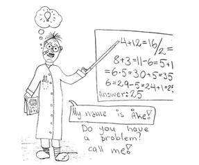
As part of research project, one of my research students is studying students’ perceptions of mathematicians and what they do. We have asked groups of students from the USA and the UK to draw a mathematician and to think of reasons for hiring a mathematician (see Picker and Berry, 2001). Figure 2 is a typical example of the student drawings.
|
|
|
|
|
|
Fig. 2: A common children's image of a mathematician |
|
The pupil wrote: “Mathematicians
have no friends (except other mathematicians)
are not married or seeing anyone
are usually fat
are very unstylish
have wrinkles in forehead from thinking so hard
have no social life whatsoever
are 30 years old
have a very short temper”
These images are fairly common from the other countries in our study: Finland, Sweden, Germany and Rumania. It is important to ask: Should we be concerned about these images? What do they say about the pupils who have them and their motivation for learning mathematics and becoming mathematicians? Where do these images come from? What do they tell us about pupils’ knowledge about what mathematicians really do? Figures 3 - 7 show further examples drawn from the research work.
Those of us who enjoy mathematics, and enjoy teaching it, would probably like to challenge and change the negative views portrayed in such images. Perhaps we need to bring into the classroom more examples of mathematics in use and mathematicians at work.
The largest finding of our study is that for pupils of this age, mathematicians and what they do are essentially invisible, with the result that pupils appear to rely on stereotypical images from the media to provide images of mathematicians when asked. Pupils believe that mathematicians do applications similar to those they have seen in their own mathematics classes, including arithmetic computation, area and perimeter, and measurement. They also believe that a mathematician’s work involves accounting, doing taxes and bills, and banking; work which they contend includes doing hard sums or hard problems; yet pupils can supply no specifics about what such problems entail.
|
|
|
|
Fig. 3: — Finland, female |
Fig. 4: Showing UK's preoccupation with testing — UK, male |
|
|
|
|
Fig. 5: The foolish mathematician — Sweden, female |
Fig. 6: The mathematician who cannot teach — US, male |


|
|
|
|
|
|
Fig. 7: The mathematician with magic powers |
|
Here are typical comments from pupils about what they think mathematicians do:
In Finland, for example, four students wrote:
“I don’t know why someone would hire a mathematician.”
Two other students wrote:
“No one is so stupid as to hire a mathematician!”
In the United States, as well, three students expressed,
“I have no idea why anyone would hire a mathematician,”
as another student confessed,
“I can’t think of any reasons.”
Still another student wrote:
“I don’t think that you would need one.”
In Sweden, among many blank answers, four students wrote that they
“Didn’t know.” “I’m not sure
of what a mathematician actually does.”
In Romania, however, students’ answers seemed to centre around their own studies and fears for doing well on the very rigorous exams they must take. A student named Lavinia wrote:
“I can only use a mathematician in the 8th grade just to put him in
my bookbag and take him to the exam with me.
ATÂT! – NOTHING ELSE!”
Another female student wrote:
“He will do my homework and go to school in my place.”
A number of the Romanian students expressed this idea of a mathematician as a sort of sorcerer’s apprentice, taking exams, doing homework, teaching “math tricks,” as a third student expressed it. This notion of a mathematician as a magician is a common theme and one that we ought to reflect upon. In other articles in this publication the magician image of mathematicians is likely to be enhanced, see for example the plenary lecture by Jean Flower on the use of dynamic geometry software to investigate a circle moving within a parabola. This was a wonderful demonstration of the power of technology to open windows onto mathematics but we need to be careful to explain the significance of such esoteric mathematics problems.
In providing the images with our survey tool, we could not have anticipated how much pupils would provide a window onto their experiences in their mathematics classes. We believe that the drawings created by the pupils contain valuable insights with significant implications for teachers, their training and their practice.
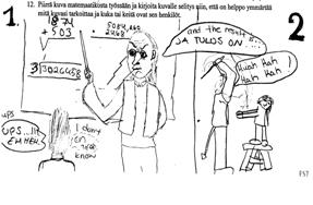
One of the most surprising and startling images pupils drew in almost every country is one of small children powerless before mathematicians who were drawn as authoritarian and threatening. Pupils appeared to use experiences of having been intimidated in mathematics classes and their criticisms of teachers for doing this, at times to depict mathematicians in their drawings in a vengeful manner, something with which they were aided by images of mathematicians in the media.
Teachers appear to be largely unaware of their pupils’ lack of knowledge about mathematicians and the role they can play both in shaping and in changing their pupils’ views about them. Solving real problems in the school curriculum can be one intervention strategy to challenge pupils' views of mathematicians and what they do and technology can give us time to reduce the 'body of knowledge and algorithms' that makes up most mathematics curricula and then do more modelling.
3 The role of technology in mathematical modelling
Clearly the power of mathematics as a problem-solving tool is not made clear to our pupils in school. I frequently ask pupils the question "What is mathematics to you?“ The common answers are numbers, algebra, and rules for doing mathematics. It is clear that most pupils believe that all mathematics is known and is made up of algorithms and rules. We have seen in the last section the invisibility of mathematics to school pupils.
Most of our curriculum in schools is focussed on developing the mathematical skills in the 'Mathematical Solution' phase of the modelling cycle shown in Figure 1. But with modern technology we can have more time to focus on the other parts of the cycle. Of course experience tells us that this is harder than just applying algorithms and I would argue that it is for this reason that we need to start modelling sooner in a pupil's mathematical career than later. In the UK the importance of 'using and applying mathematics' is an integral part of our mathematics National Curriculum and 'developing mathematical modelling skills' is an assessment object of our upper secondary curriculum. Unfortunately in primary and lower secondary schools there is little evidence of modelling skills being developed as 'investigations' and data driven models have highjacked the assessment and in upper secondary school the traditional skill based activities are the focus of the assessment. Without formally assessing the modelling process skills of Figure 1 pupils leave school poorly prepared to solve realistic problems.
Technology can be used in many ways in the mathematical modelling process. Computer simulations can be used to develop mathematical models so that students get the feel of the importance of parameters in a model. Data logging equipment provides an opportunity to collect data to validate models. Computer algebra systems can be used to 'do the mathematical problem solving part' of solving a real problem allowing time to develop the skills of formulating and revising the model. In the next two sections we look at student working styles in a modelling situation using data-logging equipment and a problem that uses the TI89 to open up a surprise in the solution to a problem.
4 Students' modelling working styles
Data logging equipment encourages an empirical modelling approach to problem solving that focuses on the shallow skills shown in Figure 8:
|
|
|
|
|
Fig. 8: Empirical modelling |
||

A curve fitting exercise allows the modeller to suggest the law obeyed by the data, and the thoughtful modeller may then suggest the origins of the parameters. The weakness of this paradigm is that a real phenomenon has to exist and to be observed in order for data to be collected before it is fitted. Its strength lies in the motivation of having observed the phenomenon and seen what it really does, allowing the mathematics to be seen as relevant and meaningful. Empirical models are often employed for prediction rather than understanding since they do not probe the underlying relationships of the phenomenon observed. Our experience of working with students, for many years, in modelling courses for undergraduates is that student working styles do not follow a systematic approach. They often fail to look back or revise their models and tend to adopt a search for data followed by data fitting to linear equations as their models. Even in open-ended problems where a theoretical approach is more appropriate many students adopt the empirical paradigm. In developing courses to develop students' mathematical modelling skills we need further empirical research to investigate students' working styles. Maull and Berry (2001) present the results of a case study of four groups of undergraduate students who were observed tackling a simple modelling task as part of an undergraduate module in mathematical modelling. This paper shows that when data-logging equipment is readily available at the start of a problem, students adopt the empirical paradigm often producing poor models.
The students were set the task of formulating a model to predict the cooling of a cup of coffee. Our first recommendation is that to facilitate students' development as good mathematical modellers, classroom instruction should promote the need to stand back initially from the actual problem at hand and to spend time at the start reflecting on the physical situation. Students should be encouraged to write down in words what is happening physically and should agree how to approach the various pieces of the jigsaw puzzle that will likely be the outcome.
Three groups adopted an empirical approach without giving much thought to the complexity or various cooling processes that might be occurring. The data gathering equipment was readily available and their behaviour was what we might consider from a group of physics students. We had provided the equipment in order to observe the students' natural strategy to solve the problem. Of course we could have initially withheld the equipment and watched them 'getting started'. The drawback of this approach is that it could have led to our early intervention and discouragement of the students' own desired method of attack.
Having collected the data it was surprising (and disappointing) to see the students’ analysis and their attempt at finding a relationship between the variables.
Here is an example of some of the dialogue between the students and the researcher (WMM). Two possible models were considered by the students: linear and exponential.
“Is it linear?”
Groups A, B and D. The first impulse of the students was to assume that the relationship would be, at least to a first approximation, linear. Some students were firmly wedded to the notion that linear is best and were prepared to sacrifice some of the empirical data to achieve this.
(Group B Time = 11.40)
S3: The graph (on a graphic calculator) looks as though it would be linear if you lose the ends.
S4: You can’t just lose the ends.
S5: Just do a graph and see what we get.
(Time = 12.15) S4: It looks not linear.
S5: Could be a bit exponential.
“If it isn’t linear then it must be exponential.”
Some students, once the notion of an exponential model had been mooted, decided quickly on appropriate steps to check the model.
(Group A Time = 11.40)
S6: You can just about see the curve (on a calculator scatter plot)
S7: When shall we stop measuring?
(Group A Time = 12.00)
S6: We think it isn’t linear.
S7: It looks exponential.
WMM: How would you check to see if it’s exponential?
S6: We could draw a log graph.
S7: Log both- no, just temperature against time.
S6: Do we use base e or 10?
Some students, although they clearly knew about exponential relations in theory, used inappropriate tools and needed more guidance towards checking their model.
(Group D Time = 12.12)
S8: It cools faster without a lid.
WMM: What do you think about the shape of the graph?
S8: This one looks exponential.
WMM: How might you check if you think it’s exponential?
S9: A log plot.
S8: Can we use Omnigraph?
(Time = 12.35) Students plotting spline curve of temperature against time on Omnigraph. They had also calculated linear and exponential regressions on a graphics calculator.
WMM: What is the form of an exponential equation?
S9: y=ex
WMM: What happens if you take logs?
S9: ln(y)=x
So what should you plot to get a straight line if it’s an exponential?
S9: Natural log of y against x
WMM: What is your y?
S9: Temperature
WMM: And your x?
S9: Time. So we plot log temperature against time.
Investigate implications
An inappropriate model gives rise to a prediction of unlikely behaviour. The students are willing to be challenged and to modify their model,
(Group B Time = 11.55)
S3: Both (cooling curves for mugs with and without lids) look linear.
WMM suggests looking along line to see if there is a curve. In fact this is difficult on LCD display because of narrow angle of view.
WMM: What will happen at room temperature if it is linear?
S4: It will go on getting cooler.
WMM: Does water do that?
S4: I don’t think so!
WMM: Do you think “It looks linear over this range” is a good enough model?
Refining the model
This group might be regarded as having successfully produced a mathematical model for the cooling of the mug of water. They have produced a first model, which they refine and from which they can now obtain numerical constants.
S7: The log thing looks nearly like a straight line.
S6: We stopped too early.
WMM: What does the temperature tend towards?
S6: Room temperature.
S7: So we could take away room temperature.
(Time = 12.40) S7: The graph of log(T-Tm) is straigh. (data plotted on graphic calculator).
WMM: Did you find the constants from it?
S7: No -here they are. Gradient is -0.0245. Intercept is 4.184. So temperature is 4.184-0.0245t.. No. ln(T-Tm) = something minus something times time. (some manipulation on paper) (T-Tm)=Ke-0.025t where K=e4.18
We would have expected that first year mathematics degree undergraduates would have the skills to quickly form a relation as a mathematical model and then reflect or criticise. To encourage a cyclic view of modelling through an experimental approach to a problem, the investigation should still consist of four phases. In the first phase, students freely explore and discuss the physical situation in order to design appropriate experiments. In the second phase students collect the data and formulate a model. The third phase consists of a comparison of the model with the physical description and features outlined in phase one. The fourth phase is a refinement of the model either by creating a different relationship (e.g. from a linear model to an exponential model for the cooling problem) or collecting new data.
What do we learn from investigating students working styles when modelling? The most important observation from the dialogue above is that the students are working in a very haphazard way. They rush in to collect data. The natural instinct because of the modelling experiences that they have learnt in school is to work on an empirical model. Our first recommendation is that to facilitate students' development as good mathematical modellers, classroom instruction should promote the need to stand back initially from the actual problem at hand and to spend time at the start reflecting on the physical situation. Students should be encouraged to write down in words what is happening physically and should agree how to approach the various pieces of the jigsaw puzzle that will likely be the outcome.
Our second recommendation is to facilitate students' development as good theoretical mathematical modellers we would recommend that data logging equipment should not be available at the outset and that students should be encouraged to discuss and explore the physical situation.
The appropriate use technology must be carefully taught to students so that it is not used poorly.
5 A resource of problems
If we are to develop good theoretical modelling skills then we need a resource bank of problems that demonstrates the mathematical skills needed and the important role of technology. I offer the following as an example.
Modelling motorway traffic jams
Traffic queues often form on motorways when three lanes of traffic are forced to reduce to two lanes or to one lane because of road-works or accidents. This is a major frustration to motorists and often extends journey times by hours.
Consider the problem of reducing two lanes of traffic to one. What speed of traffic achieves a maximum flow through the motorway section?
A full solution will not be given but the steps in the solution are outlined below: The objective is to maximise the number of cars per hour passing through the motorway section; this is the flow rate which we designate as F. Suppose that vehicles enter the section t seconds apart. Then the number of cars entering per second is 1/t and the flow rate is
![]() .
.
Suppose that the distances between the fronts of two vehicles is d metres.
At a speed of v ms-1 the quantities t, v and d are connected by the equation d = vt.
Hence the expression for the flow rate becomes
![]()
|
The distance d is made up of two parts, the length L of the vehicle and the separation between the vehicles s, so that d = s + L and the expression for the flow rate becomes
|
|
|
Fig. 9: Distance between cars |

Modelling the separation distance
The British Highway Code recommends overall safe stopping distances between vehicles for different speeds. Using the data from the Highway Code the thinking distance in feet is the same as the speed in miles per hour (u). With the aid of algebra and/or graphs it can be shown that the braking distance is u2/20. Hence,
![]()
and if we assume that all the vehicles are average sized family cars then L = 13 ft. The mathematical problem is to find a maximum of the function
The TI-89 screen for this activity gives
|
|
|
|
|
Fig. 10: Finding the solution with a TI-89 |
||
The conclusion is that the vehicles should travel at about 17 mph (or 27 km/hr on European roads!).
The next step in the modelling process is to criticize and improve the model. It is unlikely that vehicles will travel at the ‘recommended safe stopping distances’. So it is the formula for stopping distances that will need to be revised.
It is common for students to argue that the ‘thinking distance’ can be reduced or even ignored. However as we shall see this will lose some essential information.
Consider, instead, an algebraic model in which we take the separation distance as the expression
![]()
Now the mathematical problem is to find a maximum of the function
![]()
The TI-89 screen for this activity is
|
|
|
|
|
|
Fig. 11: Finding a maximum of F(v) |
|
The algebraic approach leads to the solution
![]()
(surprising for many students that the value of v for maximum flow rate is independent of the thinking distance. This example demonstrates the important skill for the mathematician of being able to investigate algebraically situations involving parameters. If one of the roles of mathematics is to explore problems, then, like statisticians who use technology to explore realistic data sets, mathematicians must start to realise that technology should be used at all levels of learning to explore more realistic problems.
6 Conclusions
In conclusion I would argue that we have much to do to reshape our school and college curricula to include mathematical modelling as an integral part at every level. There is still a strong emphasis on the algorithms and skills of the 18th and 19th centuries and the notion of a body of knowledge that all school leavers should know. The appropriate use of technology can change this view but we need to be bold!
Technology
can do the algorithms and rules part of the curriculum very well and correctly
unlike many of our students. Clearly from the example in section 5 we need to
develop good algebraic skills because these skills are important in formulating
models. But do we really need our students to be able to do all the calculus
skills by hand?
Without
the need to learn all the traditional algorithms and skills we can save time
however it is important to ensure that the school authorities do not take the
time that is saved for other things! Using technology to do the mathematics
allows us to concentrate on the difficult part of the modelling process - the
formulation phase.
Teaching
with technology provides opportunities to use more realistic problems in the
school curriculum thus opening a window onto the world of the work of
mathematicians. We can then challenge the invisibility to pupils of what
mathematicians actually do. However we need to be careful to ensure that our
use of technology does not reinforce the common perception among pupils that
mathematicians are wizards and magicians.
I finish with an extract from Kutzler (1996):
What sort of mathematics should we be teaching in the future? A new form of instruction, using tools that change both teaching and learning, would embrace the following:
Mathematics
as a problem solving art: the solution of problems is one of the foundations of
human nature, one of the skills that are used in almost every situation.
Mathematics
as a cerebral workout: in an era where computers take on much of our mental
workload, we must ensure that our intellectual powers do not atrophy.
Mathematics
as culture: mathematical and cultural developments have always occurred hand in
hand. Mathematics is an integral part of our civilization; an understanding of
mathematics helps us understand our culture.
This was published five years ago - I expect that we still have a long way to go to reshape the curriculum so that Mathematical Modelling becomes a core part with technology taking more of the strain.
References
Flower J. (2001) Fitting function families using CAS and DGS. Plenary Lecture at ICTMT 5, Klagenfurt.
Kutzler B. (1996). Improving Mathematics Teaching with DERIVE. Chartwell-Bratt, Studentlitteratur, Lund, Sweden.
Maull, W. and Berry, J.S. (2001) An Investigation of Student Working Styles in a Mathematical Modelling Activity. Teaching Mathematics and Its Applications 20 No 2, 78-88.
McCray P.D. (2001) Business View on Math in 2010 C.E. CUPM Discussion Papers about Mathematics and the Mathematical Sciences in 2010: What Should Students Know? The Mathematical Association of America.
Picker, S.H. and Berry, J.S. (2000) Investigating Pupils' Images of Mathematicians. Educ. Studies in Mathematics 43, 65-94.
Principles and Standards for School Mathematics (2000). NCTM.
Differential equations instead of analytical methods
George Adie, Bengt Löfstrand, and Bogdan Zoltowski
Kalmar, Sweden; Lodz, Poland
1. Motion in one dimension with constant force, g = 9,81 m/s2
2. Motion under gravity in two dimensions
3. Trajectory with air resistance
This paper is written by physicists from the point of view of physicists. We have written it in order to show the way in which CAS and numerical techniques are changing the way in which we teach physics to engineers at undergraduate level using differential equations instead of analytical methods. There is a symbiosis between our subjects, which means that mathematicians should know how our teaching methods are changing so that they can adapt their teaching of maths. The tradition in physics is to teach mechanics and transients in electricity using analytical equations. The truth is that these analytical methods models are applicable in less than 1% of real world situations. We can increase this level of applicability by working directly from differential equations. This has been made possible by the advent of CAS and numerical techniques. So we do it. We have already published a number of papers showing advanced versions of these methods in the study of transients. In this paper we will concentrate on dynamics so that we can highlight the continuity in this way of thinking. We will try and emphasise the continuity by introducing topics in the following order:
1. Motion in one dimension with constant force.
2. Two-dimensional motion in a parabola.
3. Two-dimensional motion in a parabola with air resistance.
4. Two-dimensional motion in a circle – vertical circle.
5. The pendulum – large angles.
6. Physical pendulum with damping.
The first two of these are standard fare for our physics courses and can be easily explained using analytical equations. We choose to use differential equations instead because it gives continuity, working up to a real situation with air resistance. Number 4 is also standard fare, but it is interesting to see how it develops naturally into cases 5 and 6, which are completely out of traditional courses.
1 Motion in one dimension with constant force, g = 9,81 m/s2
|
It is easiest to start with a simple falling body here so that the ideas can be developed towards two-dimensional trajectories and air resistance. We use Newton’s law
where m is the mass. Traditionally, this relationship is expressed using a set of (5) analytical equations. |
|
|
Fig. 1 |
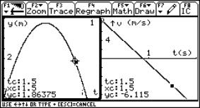
The alternative way of working is to analyse the graph written using a numerical method (such as Runge-Kutta s method). A typical question with solutions is shown below. The way in which the differential equations are fed into the calculator is shown as part of the next example.
|
A ball is thrown upwards with an initial velocity of 8.6 m/s. What is its height and velocity after 1.5 s? From the graphs, the height is 1.86 m and the velocity is –6.12 m/s. |
|
|
Fig. 2 |
2 Motion under gravity in two dimensions
The previous differential equation
![]()
applies in the vertical direction. There is no horizontal acceleration so
![]()
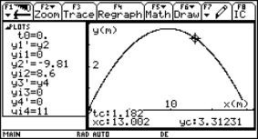
These two are fed into the calculator with initial conditions as shown below. In this case a graph showing the variation of y with x is shown together with the solution to a typical question.
|
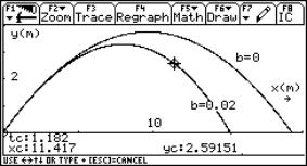
A ball is thrown in the air with initial vertical velocity 8,6 m/s and horizontal velocity 11 m/s. How long does it take to travel 13 m horizontally, and what is its height then? The answers are 1.18 s and 3.31 m as shown on the right. |
|
|
Fig. 3 |
3 Trajectory with air resistance
It can be shown using energy considerations that there is an air resistance giving a force opposed to the motion and proportional to the velocity squared.
|
F = m·b·v2 where b is a constant that depends on the form of the object. Using Newton’s law in the horizontal direction,
We can write
so
|
|
|
Fig. 4: Forces acting on the ball when its velocity makes an angle q with the horizontal |

In the vertical direction,
![]()
Using arguments similar to those in the horizontal case,
![]()
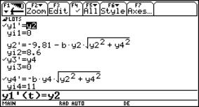
These are fed into the calculator as shown below and then the graph of y against x can be compared to the case in which there is no air resistance. In the case with air resistance here, b = 0.02 m-1. The height and horizontal displacement is taken after 1.182 s, which is the same time as in example 2.
|
|
|
||||||
|
Fig. 5a |
Fig. 5b |
4 Circular motion
|
We start with the simple case where the only force acting on the particle is the centripetal force. F. This could be tension in a string. In this case, the angular velocity
is constant as is the tension F in the string. |
|
|
Fig. 6 |
|
This means that q´´ = 0 is the simple differential equation that defines the system and the equations x = r·cosq with y = r·sinq give the x and y coordinates. x = r·cosq Þ x´ = -r·q·sinq. y = r·sinq Þ y´ = r·q·cosq. These equations are fed into the calculator as shown on the right. y1 = q, y3 = x; y4 = y. |
|
|
Fig. 7 |
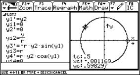
The initial conditions are chosen at q = 0 and a graph is shown of y against x with the actual position after 0.5 s. A useful pedagogic tool here is to set v = p/180 and r = 1. This way you get a unit circle from which sines and cosines can be found.
5 The vertical circle
The figure shows a small body that is being forced to follow a vertical circle by the tension F in the string. F plays no part in giving the body its tangential acceleration aT = r·q´´. It is only the tangential component of the body’s weight, m·g that has an effect on aT.
|
Using Newton’s law, m·aT = m·r·q´´ = -m·g·cosq gives us the new differential equation for q
This is easily fed into the calculator instead of the previous equation for y2´ with q´´= 0, we write
|
|
|
Fig. 8 |

|
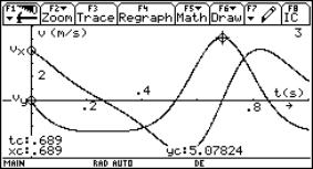
The graph of y against x is still a circle. This is not so interesting. We can look at how the velocities y´ and x´ change with time instead. Study the motion of a small body in a vertical circle with radius 0.5 m and a start velocity of 4.0 m/s where t = 0 when q = 0. What is the maximum vertical velocity and when does it occur? Answer from the graph is 5.08 m/s after 0.69 s. |
|
|
Fig. 9 |
|
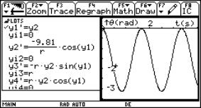
It is natural to go from here to a circular motion in which both the original angle and angular velocity is zero. The input screen together with the graph of angle against time is shown on the right. We get an oscillating pendulum. It is not simple harmonic motion. |
|
|
Fig. 10 |
6 The (physical) pendulum
|
This is not at all dissimilar from the vertical circle. It looks different because we usually measure angles from the vertical using f = 270º + q (see Fig. 11). Using the same type of reasoning as previously,
|
|
|
Fig. 11 |

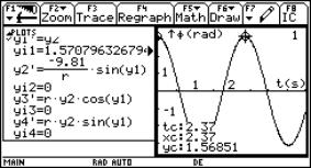
These are fed into the calculator with initial conditions with f = 90 º and the initial angular velocity 0 rad/s. (as before). The input screen and graph is shown on the right. You can see how the period is 2.37 s compared to the value 2.01 s for small angles.
Damped oscillations
|
|
|
||||||
|
Fig. 12a |
Fig. 12b |
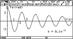
We can add a damping force that is opposed to the motion and proportional to the square of the velocity as in the trajectory case. This means changing y2´ so that it looks like
![]()
One of the possible ways of displaying the relationship is shown. This cannot be done using analytical methods.
7 Conclusions
There are a number of very important conclusions that can be drawn from this paper:
First, using these methods gives us the chance to study a large number of relationships in physics that are just not accessible using analytical methods
Second, the use of differential equations in this way gives continuity to the teaching of dynamics, from the simplest of motions with constant acceleration to complicated motions that can only be represented using numerical models.
Third, numerical methods of solving differential equations will become more important than analytical methods.
We would like to see our engineering students learn these methods of solving differential equations in mathematics instead of wasting time on the very few “solvable” cases. We would like them to be able to evaluate and judge the quality of different numerical methods in different situations.
References
Adie, G. (1998) The impact of the graphics calculator on Physics Teaching. Phys. Educ. 33 (1).
Adie, G. (1999) Graphical Calculators and Mathematics in Physics Teaching. Shaping the Future. Physics in a mathematical mood. IoP. ISBN 0 7503 0622, 33-35.
Adie, G. (2000) Using the TI-89 in Physics. bk-teachware 2000. ISBN 3-901769-31-5.
Adie. G., Zoltowski, B. (1998) Graphing calculator based activities in the student physics laboratory. XII Conf. on Teaching Physics at Technical Universities, Poznan
Adie, G. Zoltowski, B. (1999a) Differential equations in practical physics teaching. IV ICTMT, Plymouth.
Adie, G. Zoltowski, B. (1999b) Mathematical aspects of using the calculator as a demonstration tool in physics. IV ICTMT , Plymouth.
Adie, G. and Zoltowski, B. (2000a) The Impact of Handheld Technology on Physics Teaching for Engineers. PTEE 2000, Budapest Hungary.
Adie, G. and Zoltowski, B. (2000b) Handheld Technology in the Undergraduate Physics Laboratory. PTEE 2000, Budapest Hungary.
Enns and McGuire ( ) Nonlinear Physics. ISBN 0 8176 3977 2
Mullin, Tom ( ) Chaos and its application to physical systems. The nature of Chaos. ISBN 0 19 853954 1, 1-22.
Ti-89 Guidebook. Texas Instruments.
Laplace Transform and electrical circuits:
An interdisciplinary learning tool
G. Albano, C. D’Apice, and M. Desiderio
Salerno, Italy
3. Importance of Laplace Transform
The present work is addressed to high school students with scientific trend and it aims at supporting the pupils in learning two subjects: the solution of second order linear differential equations and the study of electric circuits. The two subjects are correlated because one of the presented methods to solve the differential equations uses the Laplace transform, and this is the best way to solve the integral-differential equations that are met in the study of the electric circuits. A package is created using a CAS as Mathematica. The package provides a theoretical framework and many exercises where the students are leaded step by step to solve the differential equations. Using this package the equations describing electric circuits can be solved, and consequently physical quantities evolution (current intensity and voltage) can be obtained.
1 Introduction
During the everyday life, many phenomena happen which can be explained using physical laws, but often the whole understanding of such laws requires a specific mathematical formulation. Mathematics provides some indispensable tools useful in order to interpret those laws, among such tools the differential calculus has a main role, in particular referring to the theory of the differential and integral-differential equations. The second principle of Dynamics is just an example of foregoing introduction; that principle is expressed by the equation F=ma and interpreted by a differential equation of the second order, its solution expresses the position at any time of a material point subjected to the force F.
The theory of differential equations and their solution methods is a fundamental tool in order to study the several physical phenomena. This topic is part of advanced high school (with technical or scientific addresses) curricula; it allows the students to have a better approach to all technical-scientific subjects as physics, electronic, electrotechnic and others, which make large use of such mathematical tools.
In this paper, we present a didactical software to support traditional learning process of some solution methods of differential equations; the users are driven and aided in using such methods. The software gives one of the classical examples of application of the theory of differential equations: the study of electric circuits. Such choice shows the importance of availability of many different solving methods. In general the equations that emerge in such context can be simply solved only applying the “Laplace method” and not the “classical method”. Just for such reason the solution of the differential equations related to the electric circuits are generally omitted in the school books. The creation of the software is also motivated by such lack of treatment of the topic in school books.
The key points of such work can be summarised as follows:
From a mathematical viewpoint, we introduce the Laplace Transform
method, which is useful in the resolution of the differential-integral
equations, more than the classic approach. The “Laplace Transform method” is
neglected also in advanced high school education, so it represents an
innovative element with respect to the ordinary scholastic curricula and often
it constitutes the most adapted in order to study electric circuits by
differential and differential-integral equations.
From the curricula viewpoint, we point out the interdisciplinary
approach, making the students able to understand the strong connection existing
among the different scientific subjects, introducing them to a transversal
study among the various scientific subjects and no longer sectorial. In fact, a
high level of knowledge consists not in acquiring know-how on specific subjects
(such as mathematics, physics, and so on), but in being able to connect various
concepts in order to have a more complete and real vision of some phenomena.
The student-user will be given a practical example of the interconnection
existing among the various scientific subjects such as physics, mathematics,
electronics and so on. It is clear that physics needs mathematical tools and on
the other hand the mathematics is addressed to the creation and the
investigation of techniques and tools requested by the experimental subjects.
From a didactical viewpoint, the used approach allows to start from
experience and case studies, such as circuits, and then study the mathematical
background.
The software has been realized by means of a CAS (Computer Algebra System), which mainly allows to manipulate mathematical symbolic formulas and solving symbolic calculations by using computers, typical problems of analysis, trigonometry, algebra and so on. At the beginning, such systems have been used as support to the research. At the moment they are also diffused in industry application, but above all in education as tools to teaching/learning of scientific/mathematical subjects. One of the first and actually powerful CAS is Mathematica, which is seemed the most suitable to our aim.
2 Mathematical background
The theory of differential equations and relative solution methods represents an advanced topic, which is often taught during the last classes of the advanced high school (with technical or scientific addresses). In many cases, this theory is treated just marginally because of the delay collected in teaching all the other topics or of the intrinsic difficulty of the topic itself; so in general the teaching process is just limited to an introduction of the theory of differential equations. However if the topic is studied in a sufficiently deepened way, it can give the right idea of the existing interconnection among the various scientific subjects such as physics, mathematics, electronics and so on, which are linked by mathematical foundations.
Usually students attending courses of Physics meet a wide use of differential equations, also relatively to not sophisticated topics. In such cases just the expression of solutions of the differential equations are provided to students, without giving them the explanation of the underlying mathematics needed for the solution of the considered equations. Teachers justify this due to the fact that the students lack of the fundamental notions of mathematical analysis, which should be provided by other classes. Actually, after a first step in which the students are concentrated on the physical phenomenon, it is important to have also the mathematical instruments and notion to understand analytically the same phenomenon, in order to have a deep comprehension of the subject. On the other hand, this allows the students to avoid to remember a sequence of formulas (lack of meaning by their point of view), often very hard to remember. Moreover, if this implies more notions to teach/learn, the subsequent deeper understanding, motivate the students to study and allow them to be aware of the existing connections among the various involved physical quantities and the effects resulting by variations of those quantities.
Besides the foregoing discussion agrees with the widespread idea that it is not convenient providing just the solutions of the problems to be solved to the students, but on the contrary it is necessary that they acquire knowledge and know-how needed to face generic problems and that they become able to select the most adapt method for the specific problem. From such considerations, the need of providing the adequate preparation to the students has origin; making the students able to correctly interpret and solve the differential equations should be the aim of the teaching itself. However taking into account the intrinsic difficulty of the topic, the teacher should never neglect the heterogeneous composition of the class: not all the students have the same skills, knowledge and, above all, not all of them are interested in the same measure in learning advanced topics. So the teacher must differentiate the knowledge level for each student in order to pay more attention to the ones with more difficulties and at the same time satisfying the interest of those who desire to enrich their knowledge.
The created software has just the aim of join the previous needs: it is proposed as a valid support to the understanding of the theory of the differential equations and of the circuits addressed to those students, for whom the topic is too hard. The software provides the theoretical basis in a very simple form jointly to some example in which the solution is explained step by step. On the other hand, the software represents a useful tool for more prepared students who wish enrich their knowledge.
3 Importance of Laplace Transform
Ordinary differential equations and partial differential equations are often used to solve many problems of the Physics. The born of the integral transform and their transformed and anti-transformed is strictly connected to the necessity of solving more simply these equations. The integral transform is a mathematical operator, that associates to an existent function the integral, done between two suitable extremes, of this function times a function K(t,y) (called Kernel). That is:
Integral transform:
|
|
|
|
The value of the integral transform just defined
|
|
|
|
is function of the variable y. The particular type of Kernel defines the several transforms, each with specific characteristic properties. Among the more common transforms we cite the Laplace transform, where K(t,y) = e-yt and y is a complex variable, that is:
Laplace Transform:
|
|
|
|
However there are others too, which are less common because used in specific fields of the research but are very important in the same way.
The choice of the particular transform allows the simplification of the solution of the differential equations and the translation of border condition in simple algebraic equations. When an integral transform is used, it is necessary to be able to calculate the anti-transform and we require that this procedure is not complex. Regarding the Laplace anti-transform, the computation is simple when the function, whom we want the anti-transform, is a rational fractional function with the degree of numerator less than the degree of denominator.
The Laplace method is fundamentally based on the properties of the Laplace transform applied to derivative and integral of function. For the linearity of Laplace transform we can use this transform to both the members of a differential equation in order to obtain an equation with more simple solution; the anti-transform of this solution will be the solution of the initial differential equation. For many differential equations with constant coefficient this method is equivalent to the classic one, but it seems to be more convenient in the case of differential equations obtained by practical applications, in particular it is very useful in the study of electric circuits. These circuits are described, according to their complexity, by differential or integral-differential equations deriving by Kirchhoff laws, which, combined among them, can be reduced to a less number of equations (maybe just one), but of integral-differential type if there is a condenser in the circuit.
The contemporary presence of differential and integral terms in an equation makes very difficult its solution. Some techniques are known to solve this problem. The first one, when it is possible, consists in expressing the argument of the integral in differential form, changing in this way the unknown function. In the study of the electric circuits, this technique often is applied considering the differential form of the current:
|
|
|
|
However this method can solve the problem, but determines a more complex process and moreover allows to find an unknown function different than the wanted function, with relative consequences.
Another technique consists in deriving with respect to the independent variable both the members so that the resulting equation is of differential type. Even if this method seems to be simple and fast, it requires the derivability of the coefficients of the initial equation. The latter condition is not always guaranteed: in fact in many cases the voltage of the circuit is involved and it often presents some discontinuities, so that the above technique cannot be applied in the study of the circuits.
In order to avoid such difficulties, the Laplace transform is the most appropriate mathematical tool because it just uses the integration and no particular condition are imposed on the involved functions. This justifies the importance of that transform in the analysis of the electric circuits.
4 An example
In this section we present an example in order to make clear the considerations of the previous section.
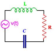
If we consider a RLC circuit, where R is the resistance, L inductance and C the condenser, q(t) the charge on the condenser and j(t) the current at the time t .
|
Given the initial data
we aim to determine the unknown function that represents the current j(t). Observing that
and using the first Kirchhoff we have
|
|
|
Fig. 1 |
This is a differential-integral equation with respect to the unknown function j(t). Deriving with respect to the variable t, a second order differential equation is obtained and this requires that the applied voltage v(t) is derivable, condition not always satisfied in real cases.
Otherwise, applying the Laplace transform method, such difficulty is avoided because possible discontinuities of v(t) do not affect in essential manner the integration operation. Denoting with capital letters the Laplace transformed functions dependent by the complex variable y, we have
![]()
and then
![]()
so it will be enough to make computation of the anti-transform of the function J(y) to determinate the solution of the previous equation of electric circuit.
5 Software description
The software has been realised as a Mathematica package. It addresses the topic of solution of differential equations connected to the study of the electric circuits in the physics and electrotechnic scenario. On one hand, it aims to facilitate and make deeper the comprehension of the solution methods of second order differential equations with constant coefficients; on the other hand, it would be a support tool for the study of the electric circuits.
So the package can be split into two parts: one dedicated to differential equation, and the other to the electric circuits connected to the Laplace transform. Each section includes a theoretical background and a practical (exercise and applications) session.
The theoretical part is structured in a hypertextual way. The topic is accessible to students who are not familiar with mathematical needed notions, but at the same time it presents other stimuli to make deeper for those who are interested in. First of all, the classical method is introduced; regarding the equations with the non-homogeneous part is of exponential or trigonometric type. Exercises are proposed both by the users and by the computer (random generated). A step-by-step solution is provided by the software. Another section treats the Laplace transform method applied to the solution of differential equations.
Finally how to use the latter method in order to study the electric circuits is shown with particular attention to the usefulness of the Laplace transform in this case. There are many admissible circuits, due to the fact that the components (resistance R, inductance L and condenser C) can be connected in series or in parallel. The related laws are explained so that the user is able to construct by himself/herself the system of differential equations suitable to describe the chosen circuit. In most of the cases, such system involves integral-differential equations, to be solved by the Laplace method.
Finally, a practical session is provided in which the students can study the behaviour of the generic RLC circuits in series and in parallel. The user can modify the numerical value of the components, of the voltage and the initial conditions of the circuit, so that this latter can be analysed in details. Starting from the two chosen circuits, any other more complex circuit can be studied.
6 Conclusions
The presented package has been realised with the aim of being a supplementary tutor, in order to support classic lecture. The new technologies allow to construct didactical tools that are flexible, allowing different approaches to the study of a subject.
References
Albano, G. , Cavallone, A., D’Apice, C., Salerno, S. (1999). Mathematica and didactical innovation. Proc. of IMS 99 – Linz, Austria.
Albano, G. D'Apice, D., Tomasiello, S. (2000) Simulating harmonic oscillator and electrical circuits: a didactical proposal. International Journal of Mathematical Education in Science and Technology. To appear.
Amerio, L. (1977) Analisi matematica con elementi di analisi funzionale. UTET .
Codegone, M. (1995 Metodi matematici per ingegneria. Zanichelli.
Feynman, Leigthon, Sands (1994) The Feynman lectures on Physics. Masson.
Ghizzetti, A., Ossicini, A. (1971) Trasformate di Laplace e calcolo simbolico. Unione Tipografico, Editrice Torinese.
Goodyear, P., Njoo, M., Hijne, H., van Berkham (1991) Learning processes. Students’ attributes and simulation. Education and computing.
Spiegel, M. R. (1965) Schaum's outline series of theory and problems of Laplace transforms. McGraw-Hill Book Company.
Spiegel, M. R. (1976) Laplace transforms. Etas Libri.
Mathematical application projects for mechanical engineers -
Concept, guidelines and examples
Burkhard Alpers
Aalen, Germany
2. Curricular embedding and accompanying activities
3. Criteria for project definitions
4. Classes of application projects
5. Worked example: Motion function for Hockenheim Motodrom
In this article, we present the concept of mathematical application projects as a means to enhance the capabilities of engineering students to use mathematics for solving problems in larger projects as well as to communicate and present mathematical content. As opposed to many case studies, we concentrate on stating criteria and project classes from which instructors can build instances (i.e. specific projects). The main goal of this paper is to facilitate the definition of new „good“ projects in a certain curricular setting.
1 Introduction
Learning and training mathematical concepts and algorithms in engineering departments of German Universities of Applied Sciences ("Fachhochschulen") usually consists of a sequence of "small steps" with "small-sized" assignments. This is necessary in order to gain familiarity without overloading students with too much complexity. But in the end, an engineer is required to use mathematics (models, software) for solving problems in larger projects as well as to communicate and present mathematical content. Without also learning this further step in mathematics education for engineers, mathematical knowledge often remains "inert" (Mandl), i.e. small chunks of knowledge are existing, but the capability of how to apply them for solving a problem is missing.
As a remedy, we introduced mathematical application projects in the third semester (Mathematics III) after students have learnt basic mathematical concepts and symbolic computation during semesters 1 and 2 in a mathematically coherent setting. The character and success of such projects heavily depends on the curricular embedding (mathematical and application field knowledge and capabilities of students) and on accompanying organizational and tutorial activities which we will describe in the next section.
In order to really achieve the objectives stated above and to avoid frustration, projects have to be defined very carefully. As Ludwig (1998) already observed, whereas articles containing descriptions of special projects or case studies are frequent (cf. for engineering mathematics: Mustoe (1999), Westermann (2000), Challis e.a. (2000), Heinrich and Janetzko (1998)), there is only few systematic work on projects. In order to pursue a more systematic approach, we present and explain several criteria which projects in our curricular setting should fulfill like openness, mathematical richness, interesting and meaningful application context, usability of mathematical software, modularity. In doing this, we take into account criteria stated by Ludwig (1998), Reichel e.a. (1991), Ernsberger (1997), and Wilkinson and Earnshaw (2000), and we compare our type of projects with those described in literature.
Defining "good" projects according to these criteria is still a time-consuming task. We therefore tried to identify classes of application projects in mechanical engineering making definition of ever new projects easier by building instances of such classes. This way, individual projects can be defined such there is no copying of work of other groups in the same class or in former classes. As a worked example for a project belonging to one of the classes we then present the project "Motion function for the Hockenheim motodrom". Finally, we discuss our experience so far.
2 Curricular embedding and accompanying activities
The mathematical part of the mechanical engineering curriculum at the Aalen University of Applied Sciences consists of three courses to be taken in semesters 1, 2, and 3, respectively. Mathematics I and II are lectured traditionally, including a written exam at the end. These courses contain the usual concepts of linear algebra and analysis. During the lectures, application modelling properties of mathematical concepts which are important in mechanical engineering are already emphasized. Moreover, an additional learning hypertext consisting of material on stress analysis and engineering mechanics as well as links to underlying mathematical concepts is offered (for a more detailed descrition cf. Alpers, 1999). Students get already an introduction to the computer algebra system Maple™, and a tutored assignment environment for mechanics is offered in Maple (cf. Alpers, 2000).
Placing projects in the third semester has the advantage that several application subjects are available making it possible to define meaningful application projects. Concepts of engineering mechanics (statics, kinematics, etc.), stress analysis, physics, and CAD are available. Mechanical configurations can be investigated in more depth mathematically. So far, the link between computation in Computer Algebra Systems (CAS) and geometrical modelling in CAD has been exploited frequently.
The theoretical content of Mathematics III consists essentially of numerical methods (numerical linear algebra, interpolation, approximation, differential equations) which often occur in application problems. These are taught at the beginning of the semester (weeks 1-5) in 14 lectures such that students have enough time for applying them in project work afterwards. Students get full credit points for providing, documenting and presenting a project solution. Guidelines for writing the documents and for preparing a presentation are given orally and as hand-out (cf. Edwards and Hamson 1989 as a guide for this). There is no longer a written exam.
There are teams of up to four students working cooperatively on one project thus fostering communication capabilities regarding mathematical concepts. Since each group works on a different project, we avoid that one group works out a solution whereas others simply copy it.
Students are expected to work approximately 20 hours each on the project such that the overall effort needed for providing a solution should not exceed 80 hours per project. This gives a rough estimate on the size of a project. Formerly, students needed this time to work on assignments and for exam preparation, so there is no additional load on the students.
All projects defined so far involve the usage of computer algebra for "easy" modelling and computation. Therefore, a short refreshing of Maple is offered and there is a student tutor helping with CAS problems. Many projects also contain modelling and production of numerical input files for a milling machine which is done using a CAD system. For larger groups, there is an additional student tutor for CAD usage, particularly for importing data computed in Maple into the CAD system. Note that before the semester starts the students have already taken a practical course on using a specific CAD system.
As far as possible, we also make use of the facilities (parts, machines) available in the departmental labs, e.g. measurement facilities, produced parts, milling machine. Moreover, we can use the central physics lab for setting up certain experiments.
The curricular setting in Wilkinson and Earnshaw (2000) who follow a similar approach introducing projects for electrical engineers, differs from ours since their projects are smaller and positioned within the first year of mathematical education. This makes our concept rather complementary than contrary to theirs.
3 Criteria for project definitions
As pointed out in the introduction, most of the articles on mathematical projects describe special projects or case studies. Besides this, Ludwig (1998) and Reichel e.a. (1991) are concerned with conceptual aspects, i.e. identification of properties and types of mathematical projects in school. Although our interest is in university projects rather than in school projects, their work is general enough to be of relevance. Ludwig (1998) provides the following classification:
Projects can have a „magnetic mode“ or a „star mode“ depending on
whether the project is centered around an application topic requiring
(„attracting“) several other areas or around a mathematical topic branching out
into several applications. Our application projects clearly belong to the first
class.
Projects can have a „reflexion structure“ if they serve to get a
deeper understanding of the meaning and applicability of already known
mathematical topics; or they can have a „projection structure“ if they serve
to develop and learn new mathematical concepts. Our projects have a reflection
structure since the mathematical topics have been treated before.
Projects have a „line mode“ if starting point and goal of the
project are clearly prescribed (and maybe steps or hints on steps are also
given, so pupils work „along the given line“); they have a „ray mode“ if only a
main topic is given and pupils can work in different directions (rays). We try
to reach a compromise in our projects: Although the project goal is given,
clarification and discussion on meaning is often required as is the case in
real engineering life. We will take this point into account in our list of
criteria below.
Reichel e.a. (1991) make a distinction between extra-mathematically and intra-mathematically motivated projects. Our projects are centered around an application topic and hence clearly belong to the first class. On a different level, Reichel distinguishes between projects which
serve
to train a mathematical topic,
develop
a mathematical topic,
make
connections between different topics,
work
on given or experimental data,
train
ways of mathematical thinking, speaking and representation,
prepare
for a later major project.
In our projects, all of the above purposes except for the second one are of relevance where the diploma thesis can be considered as the major project at the end of the study course.
Ernsberger (1997) is concerned with interdisciplinary projects during the first period of study in mechanical engineering. He states the following criteria such projects should fulfil:
problems
should be solvable within the given timeframe
there
should be at least two solution alternatives
solutions
should require the usage of many topics taught in foundational classes
projects
should not require too much knowledge, they should leave room for students‘
interest.
Our own criteria
Our own criteria are based on the above and on the curricular embedding outlined in the previous section:
The project should be concerned with an —
from a mechanical engineering point of view — interesting and meaningful
application subject
This means that an application which is important for mechanical engineers should provide the framework for the project. As mentioned above, Reichel e.a. (1991) call such projects "extra-mathematically motivated projects". Mustoe and Croft (1999) emphasizes the importance to find the right balance between „meaningful“ and „too complex and difficult“.
In mechanical engineering, mathematically "rich" topics include design of parts (curves, surfaces) or design of motion (motion curves, motion functions). In the next section we provide a set of application classes within which such topics can be identified. These projects offer a good opportunity to strengthen the connections to application classes like engineering mechanics or CAD.
The project task should include a data acquisition
phase, preferably by taking measurements in the labs
In order to enhance the connection with the real world, data which serve as input for mathematical procedures, should be acquired by real measurements in the labs which are available in a university environment. Another way could be data acquisition via the Internet for which we give an example below in section 5. Challis e.a. (2000) provides a good example for „beginning with data“.
The project should require the application of
important mathematical concepts and models
Projects should need a rich mathematical background, i.e. mathematics should play an essential role for work on a project. To make this clearer, we give an example: If a project is concerned with surface construction (say, for a part of an automobile) and the task can be achieved simply by using surface constructions available in a CAD program where no mathematical understanding is required, this would not constitute a real mathematical application project. If, on the opposite, mathematical construction of a Bezier or a spline surface and experimentation is an essential part of the project, the project would fulfill this criterion.
The project should require the application of
mathematical software like CAS or numerical programs
In their practical life, engineers will often use mathematical concepts and models within mathematical programs, which may be symbolical (computer algebra) or numerical. Therefore, it makes sense to let engineering students apply mathematical concepts and set up mathematical models using this kind of software. The software also makes it possible to handle realistic application problems which could not be dealt with using paper and pencil.
The problem description should be open, it
should not be too prescriptive wrt. the way of completion
Whereas the usual "small" assignments provide a clear "work order" and mostly serve to exercise one concept in order to gain familiarity, a project task should not describe the way how to solve the problem. It is just the task of the project group, first to clarify the task (often corresponding with tutors including the author) as is usually the case in real life: First clarify with your customer what the problem really is all about, and then think about steps, methods or models to tackle it.
The effort necessary to achieve satisfying
results must not be too large (time-adequacy)
As mentioned in the previous sections, students are assumed to work on the project for about 20 hours each. It must be possible to get to reasonable results within this timeframe. If more is required, there is the danger that students do not spend enough time on other subjects (Mathematics III has 2 hours out of 30 in the third semester). On the other hand, there should be enough work for 3 to 4 team members.
The project task should be
modular such that subtasks can be delegated to team members
It is the intention of team work on projects that project teams think about the neccessary work to be done and set up a work plan cooperatively. Project tasks should contain identifiable sub-parts which can be delegated to team members such that every team member makes a real contribution (and is forced to do so since the overall project is too much for just one or two team members to work on). This also makes it possible to include weaker students, e.g. when measurements or real production tasks in milling machines are part of the project.
It is certainly hard to define projects which fulfill all of the above criteria to full satisfaction. Ideas for projects can be collected from modelling books like Edwards and Hamson (1989) or Fowkes and Mahony (1994), or from CAS producers as in the Maple Application Center. Moreover, application colleagues can be a very valuable source since they have an immediate interest in the students working with their models. Finally, machine parts, experiments, and production machines in the labs may also be quite inspiring.
In order to ease the work of the instructor defining projects we set up several classes of mathematical application projects in mechanical engineering which help in defining individual projects.
4 Classes of application projects
In the following we describe a set of application project classes and point out why instances fulfill (at least most of) the requirements listed in the previous section. Although the class-instance-metaphor has been chosen intentionally, one should admit that defining concrete project instances from the classes below is not as easy as declaring instances in object-oriented programming languages but still needs time and some anticipating thoughts on how students might work on the project. For space reasons, we only describe one class in more detail whereas for the others just the main topics are mentioned.
Curve or surface reconstruction
Projects belonging to this class are concerned with the geometric reconstruction of parts. Such a part might be the door of a car, a formed sheet metal, the clay model of a designer part or the cross section of knife in a slicing machine. Reconstruction of existing objects is an important part in mechanical design such that the first criterion mentioned above is certainly fulfilled. The first task in reconstruction consists of measuring points which then can be used for curve or surface construction. Here, the first interesting question for students is how to take measurements (usage of available measuring instruments, point density). This is also a subtask where theoretically weaker students can do more practical work. The mathematical subjects which are needed are interpolation or approximation (preferably with splines or Bezier curves), and curves and surfaces in parameter representation which are certainly important in engineering applications. It is not possible to do the necessary calculations by hand, so the application of mathematical software is required.
As to the fifth criterion (openness), there are different degrees of openness possible here: One could simply leave it to the students which mathematical concept to use, or one could be a bit more prescriptive. This is also connected with the sixth criterion (time-adequacy): If support for a certain kind of modelling (e.g. a spline-package in Maple) is available and this is the only way to complete work within a reasonable timeframe, one might as well include it in the project description. Using existing functions in a CAS environment still gives insight in the mathematical structure of the result (e.g. cubic polynomial pieces of a spline).
A further part of the project could be to move data from the mathematical programming environment (probably a CAS or numerical program) to CAD. One could, for example, restrict oneself to modelling just curves within the mathematical problem solving environment, transfer the data via a simple ASCII file interface to a CAD program and make more sophisticated constructions in CAD (construction of surfaces through curves). Starting with a mathematical program instead of immediately using CAD has the advantage that students really work mathematically and see the mathematical construct behind the geometrical objects which is not the case if they simply click on a button named "construct spline" within the CAD environment. In a last step students can even let the CAD system produce a data file for a milling machine (if available in the lab) and let the machine produce a (small) model. Whether or not this last step is performed can also depend on the capability of the students working on the project. Constructing real parts which can even be used in lab machines (e.g. guide blade of a turbine) seems to be a great incentive particularly for strong students.
Having different subtasks like measurement, mathematical construction with CAS, and geometric construction with CAD makes it easy and necessary (!) to delegate work to team members such that each member should be involved.
Now, if an instructor wants to set up a project of this class he/she first has to find a machine part (car door, connecting rod, etc.) with some freeform geometrical properties, and then has to decide what should be modelled (surface, cross-section etc.) taking into account time-adequacy. He/she should know what measurement facilities are avialable. These can be quite simple since a high precision reconstruction is not required. Besides this, the instructor should find out (once!) the mathematical modelling support in the CAS or other program (existing procedures). He/she should also get information on simple file interfaces and modelling capabilities of the CAD program used in his/her institution.
Curve or surface synthesis
Another important task in engineering is the design of new objects, e.g. constructing the surface of a windscreen or side mirror for an automobile, or a wing profile. Additionally, some practical constraints like maximum curvature should be part of the task description. Data acquisition here could consist of measuring boundary curves or bounding boxes. Mathematical concepts to be used are again splines or Bezier curves and surfaces and their properties like curvature. Openness can be assured by giving just constraints and possibly hints on quality criteria. Basic investigation is to be performed in a CAS environment, more sophisticated investigation of surface properties should then be done with CAD. Again, there are identifiable subtasks like measurements, CAS computation, CAD investigation, and possibly production.
Motion curve and function synthesis
The design of motion is another central task in engineering. This includes motion of machine parts like sliders in packaging machines as well as motion of "free" bodies like cars or autonomous robots. Time-adequate projects can be defined in this area if simplifications are used. This will be demonstrated in more detail in the next section where a model of the Hockenheim motodrom is constructed using arcs and line segments. The mathematical concepts required here are curves in parameter representation including arcs and line segments, spline curves and more general piecewise-defined functions. Within the framework of piecewise-defined functions topics like continuity and differentiability come up quite naturally. Moreover, function synthesis as opposed to analysis yields a wide field for open experimentation, and questions concerning quality criteria or optimality also show up.
Input data for such tasks might come from the Internet (course data) or from the lab where e.g. the motion path of a robot arm around an obstacle must be determined. One could also take a toy motodrom as starting point. Defining and experimenting with course and motion function requires a mathematical program (preferably CAS) since otherwise piecewise-defined functions can hardly be handled.
Modularity and hence the possibility to delegate tasks can be achieved by identifying the main tasks: data acquisition, curve modelling, function modelling. Moreover, this can be extended by animating the motion or by even realizing it in the lab, e.g. on a toy course.
Comparison of simplified linear and exact non-linear models of mechanical configurations
In engineering mechanics, there are often simplified linear models as well as exact-non-linear models of a configuration. Take for example the pendulum which can be modelled with a linear differential equation for small angles, the deflexionof a beam or the motion of a slider-crank mechanism. Literature on engineering mechanics or colleagues lecturing the subject can provide such examples. It is often possible to improve the approximation by using higher terms in the series representation. So, here is a wide field for investigating polynomial approximations and their range of validity. Besides this, the mathematical content might include the numerical solution of differential equations. Within the labs, such configurations are often available such that the validity of a simplified model can also be checked with real experimental data (e.g. bending a ruler).
Symbolic programs are useful particularly for series representation and work with polynomials of higher degree and also for comparison with real data as well as for computing numerical solutions of differential equations.
Subtasks here are real measurements, setting up linear and non-linear models, investigation of errors, finding a simplified model within a given error bound, animation or at least visualization. If a professional program for computing such configurations is available (e.g. for multibody dynamics) it is also interesting to compare results and see which model the program uses.
Parameter-identification in mechanical configurations
Many models contain parameters that are unknown and can only be approximated using experimentation data. This is, for example, often the case for spring or damping constants. Getting experimental data from such configurations (e.g. motion data) is the starting point for an approximation process using the least squares method. If no lab experiments are available, one can also - as a substitute - produce data (e.g. a curve on paper). The projects can be open in that students have to think about what kind of data (how much and when) they need and which class of model functions for approximation is adequate. The model including the unknown constants can easily be set up with CAS, and this also holds for computing sums of squares of differences, partial derivatives and solution of the resulting linear or non-linear system. For models where some of the unknown constants are non-linear, it is often possible to use first approximative values, apply linear least squares and use the output as starting vector for non-linear least squares. It is quite obvious that a rich set of mathematical concepts can be applied in this context. For some configurations it is easy to create an animation which can be done by one team member.
Signal analysis
Signal analysis is an important part in measuring theory. Often, „noise“ has to be removed in order to reconstruct the "real" behaviour of a machine part. Another important field of application is technical acoustics. The most prominent method of analysis is the construction of approximative Fourier polynomials (DFT). For real mathematical investigation a mathematical program is required, not just an „fft-button“ of an application program.
Signals can be produced by overlapping different sine functions including high-frequency noise or they can be recorded in the lab; the resulting *.wav-file can be converted into an ASCII sample file which then is to be investigated in a mathematics program (see also the Maple Application Center for handling *.wav-files in Maple). Students have to think about sampling rates, removal of frequencies, numerical storage of the unperturbed signal. Such signals can be made audible with freeware programs or specific Maple procedures.
As to modularity, one can identify as sub-tasks: signal recording, production of numerical sample, DFT in CAS, investigation and modification of spectrum, production of output for an audio tool. As to openness, it is up to the students how to record, to experiment with sample rates, and to experiment with removal of frequencies.
Motion or signal synthesis with Fourier polynomials
In cam design, the construction of periodic functions fulfilling certain requirements is necessary (e.g., prescription of points, line segments or other functional pieces necessary for guaranteeing synchronization). For this synthesis task, approximating Fourier polynomials are used in order to avoid the occurrence of eigenfrequencies (only sine functions with frequency below the first eigenfrequency of the excited system are used). It is surprising for students how well even straight lines can be approximated with only few frequencies.
Another similar interesting field is the construction of audio signals with Fourier synthesis.
Synthesis of machine parts under certain constraints
In the design of machine parts or small constructions which is the subject of an important lecture in mechanical engineering, often parameter variation, functional dependencies (where do I gain most?) and optimisation questions are interesting. Examples can be provided by the person lecturing the subject or can be found in books on machine elements.
Means of curve, surface and volume construction in CAD programs
CAD programs contain a variety of construction methods for geometric objects (offset curves and surfaces, rotation of curves, blending, sweeping etc., cf. Marsh 1999), and during the CAD lecture just the basic ones can be dealt with. Moreover, students hardly see what is "behind the button". In mathematical projects, some of these can be investigated in more detail where CAS is an adequate computational environment. Geometric objects computed in CAS can be imported in CAD and compared with the CAD construction.
Approximative construction of parts with reduced modelling possibilities
Some production machines can only work with a reduced set of geometrical objects: An older turning lathe, for example, can only deal with polygonial cross-sections, i.e. line segments, and the milling machine can only deal with line segments or arcs. So, an interesting question with a high potential for experimentation is how to approximate a given curve (polynomial, spline, etc.) by using the available objects.
Construction of mathematical representations for interface definitions
Standardized ASCII-file interfaces in CAD (like STEP-ISO 10303, VDA-FS by the German Association of Automotive Industry) enable the description of a lot of geometrical objects (lines, polynomial curves, spline curves etc.). Such objects can be computed in a CAS (or numerical) environment, written into a file adhering to the standard under consideration, and read into a CAD program. Here again, CAS and CAD plots can be compared.
5 Worked example: Motion function for Hockenheim Motodrom
The project description handed out to the student group had the following content:
Project: Hockenheim Motodrom
„Model the Hockenheim motodrom mathematically and construct a reasonable motion function taking into account realistic restrictions. Provide a simple animation with Maple.“
This project clearly belongs to class “Motion curve and function synthesis” although the curve synthesis is not free since the Hockenheimring should be modelled. Students started with the data aqcuisition phase which mainly consisted of getting course and related data from Internet sites; here: http://www.hockenheimring.de/. In particular, they retrieved a simple course model consisting of line segments and arcs (so width was not modelled which is reasonable for reducing complexity). They first used this data for reconstructing the course with a CAD system since they were already accustomed to constructing cross-sections using line segments and arcs. Using these objects in CAD and setting up a mathematical representation in CAS are quite different. For the latter, the mathematical concept to be used are curves in parameter representation. Students had to retrieve their knowledge on lines and arcs in parameter representation: line segments between two points are usually constructed with a parameter running from 0 to 1 and arcs by running through the angle section. In the next step, they had to construct a piecewise-defined curve with just one running parameter, so students had to think about re-parameterization. For later construction of a motion function and animation, arc-length parameterization is the most useful one but at this stage this is not necessary. The resulting curve with some simplifications (not all chicanes are modelled) is shown below.
For constructing a reasonable motion function, first realistic constraints had to be identified. These can also be found in the Internet. Students decided to use information on maximum velocity in curves (depending on the radius), maximum velocity of the car, and maximum positive and negative acceleration. They worked with a simple model where only full positive or negative accelleration was allowed, and made use of their kinematics knowledge learnt in engineering mechanics. They constructed the function v(s) (velocity depending on distance) using constant accelleration a0 which is in general given by
![]()
(v0 and s0 are initial velocity and distance resp.). The challenge here is to construct the parts in such a way that accelleration is stopped early enough such that the maximum velocity allowed is not exceeded. So, students really had to „construct with functions“ even if the functions under consideration (square root and constant functions) are simple. The resulting function is shown below. The last step then was to compute the distance function s(t) from v(s) which is also treated in the engineering mechanics class. Here, first t(s) is computed using
This function is invertible since in Formula 1 going back is only reasonable if you ended up in the gravel but driver mistakes are not modelled here! Having the motion function s(t), one can compute the lap time. This is an important point for controlling whether or not the modelling and the simplifications are adequate since lap times are also given as empirical data. It turned out that the lap time of the constructed motion function was a few seconds better than the empirical lap times which is a satisfying result.
Finally, to get an optical representation and control, a Maple animation was set up by letting a small circle move around the course according to the motion function. Here, as well as for constructing the piecewise-defined course curve and motion function, the usage of a mathematics program, preferably a CAS, is inevitable.
Three students worked on the project, one using CAD modelling, one constructing the curve and the animation and the last one working on the motion function in CAS, so the delegation aspect was satisfactorily realized. Yet, students worked more than the envisaged 20 hours each, particularly on the CAS part.
Although the mathematics needed for this project is not particularly difficult, students realized how to apply it and got a much deeper understanding of parameterization and piecewise-defined functions which is an important topic in engineering modelling.
|
|
|
|
Fig. 1: Hockenheim Motodrom |
Fig. 2: Motion function |
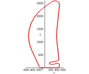
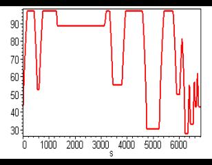
6 Discussion and conclusions
In the summer term 2000, there were 11 students working on 3 projects, in the winter term 2000/01 59 students working on 16 projects. In general, motivation was good to very high, only one group out of 16 did not manage to finish the project. A positive aspect of projects defined according to the criteria stated in section 3 is that students either really work on and are committed to such a project and then succeed (with help) or they will fail. So there is no „quick getting through“, avoiding the effect that students learn heavily one week before an exam just to forget it with the same speed afterwards.
The author as instructor had several meetings with project groups for clarification of tasks, mathematical content, how to proceed and split work, and discussion about reasonable project simplifications and restrictions. The author acted as „customer“ the students had to cooperate with and to satisfy somewhat resembling the real world of a practising engineer.
The reaction of students was in general positive but some complained about the workload, partially stemming from unequal distribution of work within groups, partially because the projects were rather challenging whereas small-sized assignments and exams were familiar and easier to handle. This applies particularly to weaker students who needed more help and hints, whereas stronger students rather appreciated the bigger challenge and often worked much more than required. But also the weaker students got a better understanding of applying mathematics and were content at the end when they managed to come to a result.
When setting up the project tasks for the summer term 2001 (9 projects) and the winter term 01/02 (20 projects), the criteria and classes outlined in sections 3 and 4 were both applied and further developped. Having made criteria clear and having a set of classes made the project definition considerably easier but this task is still time-consuming. The author intends to make a (growing) set of project class and instance descriptions available via the Internet. It would also be helpful to set up a common library of projects and project classes as was suggested by Challis e.a. (2000).
References
Alpers, B. (1999) Combining hypertext and computer algebra to interconnect engineering subjects and mathematics. Proc. 4th Int. Conf. On Technology in Math. Teaching (ICTMT 4), Plymouth.
Alpers, B. (2000) Intelligent Assignment Environments for Mechanical Engineering with Computer Algebra, preprint.
Challis, N., Gretton, H., Pitt, D. (2000) Begin with Data, End with Understanding: a Real and a Modelled Double Pendulum. Hibberd, S., Mustoe, L. (eds.): The Mathematical Education of Engineers III , Proc. IMA Conference, 139-144.
Edwards, D., Hamson, M. (1989) Guide to Mathematical Modelling. MacMillan, London.
Ernsberger, K. (1997) Erste Gehversuche als Ingenieur. Entdecken des Ingenieurberufsbildes im Studium durch interdisziplinäres Training in den Grundlagenfächern, Handbuch Hochschullehre: Informationen und Handreichungen aus der Praxis für die Hochschullehre, NI C 1.1. Bonn, Raabe-Verlag, 1-20.
Fowkes, N.D., Mahony, J.J. (1994) An Introduction to Mathematical Modelling. Wiley, Chichester.
Heinrich, E., Janetzko, H.-D. (1998) Mathematica: Vom Problem zum Programm. Modellbildung für Ingenieure und Naturwissenschaftler. Vieweg, Braunschweig.
Ludwig, M. (1998) Projekte im Mathematikunterricht des Gymnasiums. Franzbecker, Hildesheim.
Maple Application Centre: http://www.mapleapps.com/
Marsh, D. (1999) Applied Geometry for Computer Graphics and CAD. Springer, London.
Mustoe, L.R., Croft, A.C.(1999) Motivating Engineering Students by Using Modern Case Studies. Int. Journal of Engineering Education, Special Issue on Math. Education for Engineers. Tempus, Dublin, Vol. 15, No. 6, 469-476.
Reichel, H.-C., Humenberger, J., Hanisch, G.(1991) Fachbereichsarbeiten und Projekte im Mathematikunterricht: mit Anregungen für das Wahlpflichfach. Hölder-Pichler-Tempsky, Wien.
Westermann, Th. (2000) Teaching Mathematics Using a Computer Algebra. The Int. Journal of Computer Algebra in Math. Education 7, No. 4, 277-293.
Wilkinson, J.A., Earnshaw, H. (2000) Embedding Mathematical Skills for Engineers: Projects for Engineering Mathematics, Hibberd, S., Mustoe, L. (eds.): The Mathematical Education of Engineers III , Proc. IMA Conf. April 2000, 133-138.
Cross curriculum teaching and experimenting
in math & science courses using New Technology
Brigitta Aspetsberger and Klaus Aspetsberger
Linz, Austria
Cross curriculum teaching and learning by experimenting are important objectives for future math & science courses. Various practical as well as mathematical skills of the students are trained by carrying out experiments, analysing the results and finally using functions for fitting data points obtained by the experiments. The students have to combine knowledge about different types of functions with knowledge about chemical and physical theorems. As an additional aspect, the students also have to take care of accuracy in experimenting for obtaining good results.
The collection of large lists of experimental data is supported by the TI-CBL system. Mathematical experimenting, complicated computations and visualisation are supported by the graphic pocket calculator TI-92.
We report about the experiences made with several groups of students at the age of 17 to 18 and about one group of high ability students at the age of 14. Skills and abilities of the students for carrying out the experiments and for documenting the results are discussed as well as the experiences made by the teachers when working in teams.
1 Introduction
In traditional math courses the students often do not see the necessity for introducing new mathematical concepts. Examples demonstrating the application of these concepts sometimes seem to be very artificial for the students. Interpreting the results of mathematical reasoning is also quite complicated for the students if they are not able to see the physical and chemical laws underlying the examples treated.
In science courses students sometimes do not understand the meaning of the formal mathematical description of laws. They are unable to see the interdependencies of experimental data and to recognise the mathematical structure of fitting functions. Experiments carried out by students are very motivating for them and lead to a better understanding of principles and process in sciences. Furthermore, these experiments foster various practical as well as mathematical skills from the students.
Cross curriculum reasoning, the understanding and applying of laws and principles of physics, chemistry and biology as well as the possibility of describing processes and interdependencies by mathematical functions and expressions are very important goals in modern science education.
Graphic pocket calculators like TI-92 from Texas Instruments help to visualise data, to plot graphs and to execute tedious and complicated calculations like determining regression curves. Experimental data can be investigated and visualised quite comfortable by using the TI-92. The main problem is to obtain a large set of experimental data of high accuracy.
CBL from Texas Instruments is a Calculator Based Laboratory which allows to collect data during physical and chemical experiments. Data are stored directly to a calculator e.g. the TI-92 for graphical visualisation and further manipulation. CBR from Texas Instruments is a motion detector which allows to gather a large amount of data points from an object in motion. CBL, CBR and TI-92 support data collection and manipulation. However careful experimenting is absolutely important for obtaining good quantitative results, which are necessary for functional modelling of experimental data.
We report about experiments being carried out at the Bundesrealgymnasium Landwiedstrasse, which is an Austrian Grammar school in Linz in the years 1999 until 2001. In eight different groups consisting of students at the age of 16 to 18 experimenting with the CBL and TI-92 was integrated within regular classes (see Aspetsberger 1999). About 50% of the students were girls. A special course for high ability students at the age of 14 was installed during the school year 2000/01 also carrying out experiments with CBL. In 2000 a group of students were testing the water quality in regular classes using CBL and ion selective probes from Vernier.
2 Experiments
Many experiments from chemistry using CBL can be found in Holmquist, Randall, and Volz (1998) with very detailed descriptions. In the following we describe one experiment for demonstration:
In this experiment the students had to determine the concentration of an unknown green coloured solution. According Lambert Beer´s Law light absorption is direct proportional to the concentration of the solution. The students had to make a sequence of different solutions from a stock solution of known concentration and to measure their light absorption using a colorimeter. Due to Beer´s Law the concentration/absorption data points lie on a straight line. Now the students had to determine a regression line by hand or automatically by using the pocket calculator. Obtaining an almost homogeneous straight line indicates the accuracy of the sequence of different solutions produced by the students. Next the students had to measure the absorption of light of the unknown solution and to determine its concentration using the regression line by hand calculation or from the graph directly (see Fig. 1). Note the steady change of mathematical reasoning, chemical interpretations and practical work in this example.

![]()
Concentration

![]()
![]()
![]()
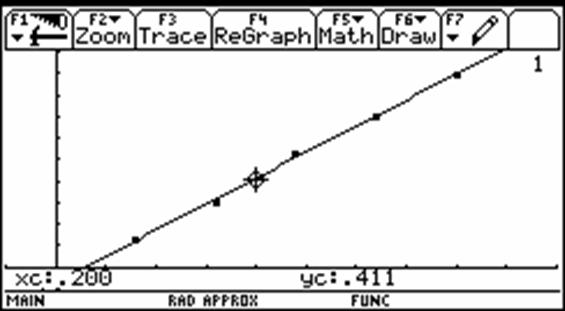
Fig 1: Determining the concentration of an unknown solution using Beer´s Law
In traditional physics courses it is very complicated or almost impossible to investigate the movement of a body in motion by measuring the distance of the body according to time. Using the CBR of Texas Instruments it is very convenient to obtain a big list of (distance/time) - pairs describing the motion of a body. Fitting data points by functions lead to a mathematical description and analysis of several processes of motion (see Texas Instruments 1997).
Being familiar with the handling of the CBL and TI-92 the students analysed the quality of freshwater (see Johnson, Holman, and Holmquist 1999) by using ion selective probes of Vernier in laboratory and outside. An intensive and very accurate calibrating of the probes was absolutely necessary for obtaining good results. This was completely new for the students. On the other hand having good calibration values it was really easy to measure the concentration of several ions in freshwater. Having only single point measurements there was no sense for a mathematical analysis. It was much more interesting to interpret the results and to compare them with official limits. Furthermore the students learned about the methods of how to analyse freshwater. Visiting the local institution for freshwater control the pupils learned that the same methods were used there.
3 Cross curriculum teaching
Experimenting with the CBL, CBR and the TI-92 (or comparable graphic calculators) requires and trains several basic skills in different areas, e.g. mathematical skills, verbal skills, practical skills and social skills (see Aspetsberger 2000 a).
The main basic skill in mathematics is the ability of recognising the functional interdependency of experimental data and to find suitable fitting functions (see Aspetsberger 2000 b). Concerning the use of the TI-92 during experimenting a secure handling of the various windows for the different representations of data is necessary.
The students have to know about the specific laws in physics, chemistry and natural sciences and how to apply them in special situations. This is very important when interpreting the results and the meaning of the occurring parameters in fitting functions.
It was surprising how difficult it is for the students to read and carry out instructions stepwise without additional explanations of the teacher. However it was much more unfamiliar for the students to document their work writing reports and interpreting the results obtained. This is really an important skill which the students have to learn. Thus, there is also a verbal component of cross curriculum teaching when experimenting in science courses.
Finally the students have to learn some practical and social skills when experimenting in groups. Experimenting in science and math courses is a good training for the multiple intelligences (Gardner 1993) of the students.
4 Experiences
The students were really motivated. According to questionnaires and feedback forms they enjoyed practical work and felt free of the “pressure of learning”. Some of the students also mentioned the importance of learning how to use technical instruments.
We forced the students to document their work and their results. However they were not happy to write protocols. They had to learn how to write reports first. Writing summaries of the experiments they understood the background of the respective experiments and some of the students wished to repeat the experiments to obtain better results.
The major problem was the lack of time. We had only 50 minutes lessons for explaining and executing the experiments. The discussion and interpretation of the results had to be delegated to the next lesson, which sometimes was one week latter. This lead to a loose of actuality.
Interpreting results was especially difficult for the pupils in the course of testing water quality. It was very hard to estimate the accuracy of the results obtained by the CBL-system. The students were not familiar with the necessity of calibrating the probes and they noted down all (senseless) digits of the results indicated on the display.
In the course for high ability students the pupils had difficulties to read the instructions in English. This was too long and boring for them. The question „What shall we do?“ was often heard. They liked experimenting with CBL and the TI-92. The necessity of writing reports was not evident for the pupils. As there was no grading for this course the pupils did not see the importance of writing protocols. Half of the group was very interested in finding new solutions and new experiments. Due to a feed back form the pupils found the course was informational and interesting.
Completely new was the role of the teachers. We were testing team-teaching – one teacher responsible for biology and chemistry and the second one responsible for math and physics. The students appreciated independent working – the teachers were only assistants and watching the students.
It was also new for the students to work in groups. They had to dedicate work to different group members according to their abilities. The second problem was to accept a unique grade for the whole group. Finally, it was quite difficult to find a fair grading for the students according to their individual achievements.
References
Aspetsberger, B., Aspetsberger, K. (1999) Integrating Math to Science Courses using TI-92 and TI-CBL. ICTCM, Int. Conf. on Technology in Collegiate Mathematics 1999, San Francisco.
Aspetsberger B., Aspetsberger K. (2000a) Experiences with CBL and the TI-92 in Austrian High School Classes. Integrating Math, Physics and Chemistry. 6th ACDCA Summer Academy 2000, Portoroz, Slovenia.
Aspetsberger B., Aspetsberger K. (2000b) Functional Modelling of Experimental Data in Science Courses. ICTCM, Int. Conf. on Technology in Collegiate Mathematics 2000, Atlanta.
Gardner H. (1993) Frames of Mind. The Theory of Multiple Intelligences. Fontana Press, London, An Imprint of Harper Collins Publishers, Second Edition.
Holmquist D.D., Randall J., Volz D.L. (1998) Chemistry with CBLTM. Chemistry Experiments Using Vernier Sensors with TI Graphing Calculators and the CBL System. Vernier Software, 8565 S.W. Beaverton-Hillsdale Hwy., Portland, Oregon.
Johnson, R.L., Holman S., Holmquist D.D. (1999) Water Quality with CBL. Vernier Software, 8565 S.W. Beaverton-Hillsdale Hwy., Portland, Oregon.
Texas Instruments (1997) Einführung in die Verwendung des CBRTM mit 5 Schülerexperimenten. Texas Instruments.
Mathematical modelling with the use of Cabri
Per Broman
Dalarna, Sweden
Click here for an interactive version of the paper.
1. The parabola and its directrix
2. A simple way to form conics
4. A rectangle inscribed in an acute angled triangle
1 The parabola and its directrix
My first example shows a very standard way to construct a parabola by using a focus point and a directrix line. Not least does this method give understanding of the reflection properties of the parabola that is hard to show in "classical" ways.
Definition: A parabola is the set of points that are equidistant from a point, called the focus point, and a line, called the directrix or the directrix line.
|
|
|
|
|
Fig. 1 |
||
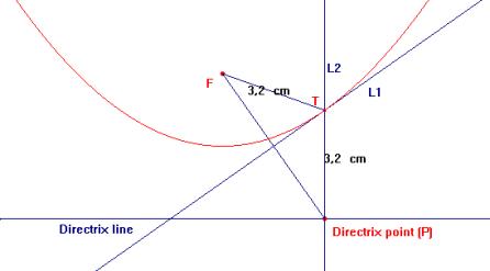
To do and explore
First we can see how this image was formed: (This works in the CD-version of the proceedings, since the images there are interactive.) Double click the image, and use the bottom menu to follow the construction. I started with the point F and then the directrix line. The directrix point sits on the line. A line segment is drawn from F to the directrix point, and a perpendicular bisector, L1, to this segment. L2 is constructed through the directrix point perpendicular to the directrix line. The point T is the intersection between L1 and L2. Now the locus of T as I move the directrix point is a parabola, which we will see. L1 is always a tangent line to the parabola.
Since L1 is a perpendicular bisector of FP, the triangle FTP has two legs equal. According to our definition, the locus is a parabola. Note, that the opposite angles between L1 and L2 are equal, and therefore the angle between the line segment FT and L1 also equals the angle between the lines. If L2 is an incoming ray that is reflected in the parabola, it will be reflected towards F.
2 A simple way to form conics
|
The image is constructed the following way (see Fig. 2 and 3); the point P runs freely on the blue line. The line L1 is perpendicular to the segment FP. If I use the “Trace On” in Cabri on the line L1, and the animation spring on point P, I will get the following image: The envelope of L1 as P moves along the blue line is a parabola (which can be proved by for example the fact that the blue line would lay exactly half way between F and a directrix line). |
|
|
Fig. 2 |
|
|
|
|
|
Fig. 3 |
|
|
There is a similar way to form the other conic figures, the ellipse and the hyperbola. We use a circle instead of a line and construct a line L1 perpendicular to the segment FP (as before; see Fig. 4). |
|
|
Fig. 4 |
|
|
By using trace and the animation spring, we can see that the envelope of L1 is an ellipse (see Fig. 5) |
|
|
Fig. 5 |
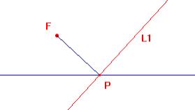
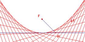
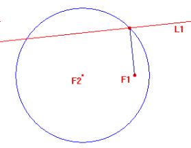
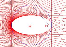
|
If we do the same thing as before, but with the point F1 outside the circle, we get a hyperbola (Fig. 6) We could regard a line as a circle with infinite radius. Then a point which is not on the line-circle could be regarded as inside and outside the circle simultaneously. Thus, the parabola can bee seen as the very limit between ellipse and hyperbola. |
|
|
|
Fig. 6 |
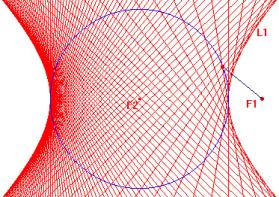
3 The directrix circle
This last example gave me the idea to look for something corresponding to the directrix line of the parabola. What I found was directrix circles for the other conics. A little bit to my surprise the very same construction that gives an ellipse, also gives a hyperbola. Also here the reflection properties come out very nicely.
|
Definitions: An ellipse is the set of points T such that the sum of the segments F1T and F2T is constant. A hyperbola is the set of points T such that the absolute value of the difference between F1T and F2T is constant. F1 and F2 are two points. The directrix circle has its origin in F1. P is a point on the circle. L1 is the perpendicular bisector of F2P. L2 is a line through F1 and P, and T is the intersection point between L1 and L2. The ellipse is the locus of T as P moves. |
|
|
Fig. 7 |
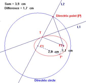
Now, F1T + TF2 = F1P = the radius of the circle, and hence constant. According to the definition we prove that the ellipse really is an ellipse.
|
Here, as in the parabola case, we need just simple geometry and the fact that L1 is a tangent line to the ellipse to show that a ray F2T will be reflected towards F1. Simply moving F2 outside the circle forms this next image. In this case |F2T – TF1| = |PT – TF1|, why the locus really is a hyperbola. We can also easily see that a ray from F2 towards T will be reflected away from F1. The opposite is also true, but we need to use the image dynamically to see that as easily. |
|
|
Fig. 8 |
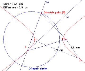
4 A rectangle inscribed in an acute angled triangle
This title gives a problem of enormous richness:
|
The construction is briefly constructed like this: T is a point on the side BC. The rectangle is constructed out of that point. The base of the rectangle is set off on the x-axes, and the area of the rectangle on the y-axis. The intersection of the thin blue lines give a point, and its locus as we move t gives a curve we can measure. It is a parabola! |
|
|
Fig. 9 |
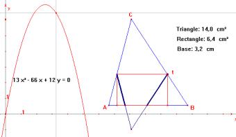
The rectangle has its maximum as t is halfway between B and C, and the maximum area is exactly half of the triangle area. The reflected line segments in the rectangle part of the image show why, especially if you work with the image dynamically.
If you move the point C sideways, this will not affect the area function. As long as AB is constant, the area function is not dependent on the shape of the triangle, only on its size.
Normally a function works like this: You can vary x, and that will affect the value of y. In this case we want a graph of x and y, but we vary a parameter t. I think this is a good example how to introduce the concept of parameters.
Modelling human growth
André Heck and André Holleman
Amsterdam, The Netherlands
4. Further investigation: The ICP-model
We have used the recent Dutch growth study to create learning material for pupils in the second stage of pre-university education (age 15-18 yr.) to carry out practical investigation tasks. We shall present the learning material and discuss the classroom experiences.
1 Introduction
Body growth of children is often used in mathematics textbooks as an example for discussing processes of change, statistics, and discrete and dynamical models of growth. However, the real world context is in many exercises only used for ‘dressing up’ a mathematical problem or as an ‘ideal’ illustration of a mathematical concept.
|
In Figure 1, we show the real diagrams of mean height and increase of mean height for Dutch boys together with a textbook example of a boy called Hank. How credible is Hank’s growth curve? |
|
|
Fig.1: Real and artificial growth curves |
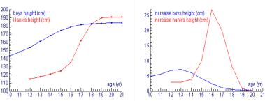
One may argue that real data are too unmanageable or distracting for successful introduction of a mathematical subject. But this argument does not hold anymore when it comes to applications of mathematics by pupils in real contexts, assuming that the pupils have convenient tools to collect, to process, and to analyse real data. In our research we examine the possible contribution of ICT and context situations to the realisation of challenging mathematical investigation tasks for pupils. It provides input for the ongoing development of the learning environment Coach (Heck 1999) and learning materials for pupils that stimulate and enable them to carry out mathematical investigation tasks at a rather high level. Software and pupils’ activities are tested in practice.
2 The learning material
The learning material is designed for pupils who are in their first year of the second stage of pre-university education (age 15-16 yr.), who have no experience with practical investigation tasks, and who have not worked with Coach before. Our main objectives are to let the pupils
work with real data and with diagrams that are
actually used in health care;
experience how much useful information can
actually be obtained from diagrams;
see that the change of a quantity is often as
important and interesting as the quantity itself;
practice ICT-skills;
carry out practical work in which they can apply
much of their mathematical knowledge.
The learning material is based on medical literature, especially on documents that describe the growth data and the results of the 4th Dutch survey (Wit 1998). English versions of the assignments can be downloaded from http://www.science.uva.nl/~heck/research/growth/
Estimated study load is 6 to 8 hours. First, pupils carry out the following three assignments:
1. The Dutch Growth Study of 1997. A quiz gives the pupils an idea of how much they already know about body growth and puberty. We use a newspaper article to introduce the 4th nation-wide growth study and to illustrate the relevance of growth data.
2. Mean Height Growth. Pupils get familiar with the main tools of Coach for studying human growth. They learn how to make data plots and increase diagrams of height in relation to age, and they learn how to interpret these diagrams in the context of child growth.
3. Secular Height Growth in 1980-1997. Pupils use the data from the Dutch surveys of 1980 and 1997 to study the changes in mean height for Dutch children in this period.
Finally, pupils select one of the following subjects to investigate by themselves:
A. Growth Charts of Native Dutch Children. Pupils learn how growth charts are made, what they mean, and how they are used. They also compare their own data with their peer group.
B. Mathematical Model of Height Growth for Girls. Pupils compare the mean height growth for girls with Turner syndrome with the growth for healthy girls and they make a simple mathematical model of the height growth for girls until puberty.
C. Mean Weight Growth. Pupils investigate the mean weight growth for healthy Dutch boys and girls in relation to age. They search for points in common and for differences, and they make a simple mathematical model of weight-for-age for children until puberty.
D. Mathematical Weight-for-Height Model. Pupils investigate the mean weight growth for Dutch children in relation to height and make a mathematical model of weight-for-stature.
|
The main role of ICT in the activities is to visualise, process, and analyse real data. On the left-hand side of Figure 2 are the diagrams of mean height growth for Dutch children in relation to their age and the corresponding increase diagrams. Two things catch the eye: the growth spurt during puberty and the fact that this occurs for boys later than for girls, and with higher intensity. More differences in body growth between boys and girls can be read off. |
|
|
Fig. 2: Mean height and increase in mean height for Dutch children |
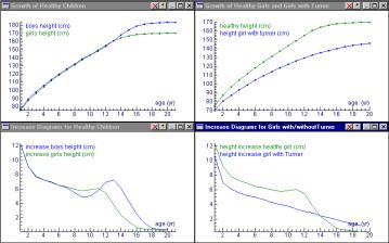
The diagrams on the right-hand side of Figure 2 are about mean height growth of healthy girls and girls with Turner syndrome. They reveal two symptoms of Turner syndrome: slow growth and no pubertal growth spurt. For girls with Turner syndrome the growth rate is after 3 years almost a linear function of age. This means that the graph of the mean height for girls with Turner syndrome is a parabola. Actually, the quadratic model describes it up to a millimetre. Who still dares to say that working with real data in mathematics lessons is too troublesome? In the assignments, pupils do similar experimental modelling of growth curves.
3 The classroom experiment
The experiment took place in a class of 26 pupils working in pairs. In the first week, work took mainly place in the computer lab during the regular mathematics lessons. In the second week, the pupils could make use of the computer facilities at school to continue all by themselves. They had to hand in the report of their work (written with a text editor), a questionnaire, and a diskette with their Coach activities and results. Together with the classroom observations and video recordings, these materials give us an impression of what the pupils actually do and of how they experience the work. Below, we list our main findings.
The strongest impression makes the good quality of the pupils’ work in general. For example, Linda and Joni describe the difference in height and height increase between girls with Turner syndrome and healthy girls as follows: “The difference in height for girls with and without Turner syndrome is not so big until the age of two. You can also see that they skip puberty more or less. Where a healthy girl starts growing faster during puberty and you can see a peak in the diagram, this is not the case for girls with Turner syndrome. They grow as it were constant.” Clearly, these pupils make good sense of the diagrams.
The abilities of pupils to create and interpret graphs have been focus of numerous research studies (Leinhardt e.a. 1990 and references therein). What we observe in our group of pupils is that they usually have no problems with interpretation tasks up to intermediate level. However, we notice that they are not used to think of change of a quantity as an interesting quantity itself.
Pupils get quickly familiar with Coach. They like the easy way to create graphs from tables and to copy results into their report. Some pupils report difficulties with getting the graphs exactly in the way they want them: choosing unique names for quantities and labelling axes are the biggest problems. Coach has a function-fit tool that enables pupils to work with various regression models. We see that they feel free to try any function type in the tool. But, when asked a simple function-fit, most pupils interpret this as a fit with a straight line.
All pupils indicate that they like it that they may choose the last assignment. Some admit that they choose the task that they guess will be easiest, others (mostly girls) give more personal reasons. For example, Linda and Joni write: “Turner syndrome looks to us an interesting subject. You have to compute something about girls and then it is nice to see if it matches with yourself.” None of the pupils find the assignments easy, but their biggest complaint is that time was too short. Some pupils prefer the normal mathematics lessons in which the teacher is always around to help them; others enjoy the freedom in this kind of activities or like the subject. We quote Inge and Annemieke: “It was fun to do; something different from the textbook and an interesting subject.” In comparison with boys, girls seem to be more interested in the subject of body growth, they pay more attention to the report, and they perform in general better. In this practical work, weak pupils also have a chance to do better.
4 Further investigation: The ICP-model
One can hardly expect that pupils discover a mathematical model for height growth in relation to age by themselves. But it is already nice if they can validate a proposed mathematical model. A fine model to test is the infancy-childhood-puberty (ICP)-model (Karlberg 1989). This model breaks down growth mathematically into three partly superimposed components:
1 Infancy (0-3 years). Restricted growth, in which the growth rate is a linear function with respect to height. It is represented by the modified exponential curve (the symbol t stands for age):
![]()
2 Childhood (from 3 years of age to the onset of puberty). A simple quadratic function fits growth during this period very well:
![]()
3 Puberty. The contribution of the pubertal growth spurt to the final height can be modelled using a logistic function:
![]()
Here, a1, b1, c1, a2, b2, c2, a3, b3, c3 are positive parameters, which must be estimated from the growth data. The mean height for each age is given by H = H1 + H2 + H3..
One can use the following curve fitting procedure. First, begin searching for a parabola that on the one hand fits well the height between 3 and 10 years of age, and that on the other hand reaches its maximum at the age of 20 years, when height growth usually stops. This curve fitting process is supported in Coach by a manual function fit. After subtraction of the extrapolated values of the childhood component from the observed values during the periods before and after this phase, two additional components are extracted and modelled. The results for Dutch boys and girls are:
|
Boys: |
|
|
|
|
Girls: |
|
|
|
The difference between computed and measured values of mean height for Dutch boys turns out to be everywhere less than 0.5 centimetres! This is a beautiful result for a formula that is completely built up from mathematical models that are studied at school. The same model can be successfully applied to weight in relation to age.
References
Heck, A. (2000) Coach: an environment where mathematics meets science and technology. W. Maull, W. and Sharp, J. (eds.). Proc. ICTMT 4, Plymouth 1999. CD-ROM published by the Univ. of Plymouth. URL: http://www.tech.plymouth.ac.uk/maths/CTMHOME/ictmt4/P75_Heck.pdf
Karlberg, J. (1989) A biologically-oriented mathematical model (ICP) for human growth. Acta Paediatrica Scandinavia 350: 70-94.
Leinhardt, G. et al. (1990) Functions, Graphs, and Graphing: Tasks, Learning, and Teaching. Review of Educational Research 60 (1), 1-64.
Wit, J.M. (1998) De vierde landelijke groeistudie. Boerhave Commissie, Leiden.
Investigating bridges and hanging chains
André Heck and André Holleman
Amsterdam, The Netherlands
Almost everywhere you can come across hanging chains and cables. Examples are necklaces, power lines, and cables that support a bridge surface. Do these cables all hang in the same mathematical shape? The first thought of many a pupil will be: this is a parabola, isn't it? In the computer learning environment Coach you can easily measure this on digital images. It will turn out that the parabolic shape quite often occurs with bridges, but that an ordinary chain does not hang as a parabola. Can this be understood? We shall show that a key idea for solving the problem can be discovered by measuring on digital images and that this can be theoretically explained with basic physics. It also leads to a simple computer model of hanging chains. We shall discuss our learning material and classroom experiences, and in this way present an example of how ICT and context situations can contribute to the realisation of challenging cross-disciplinary investigation tasks.
1 Introduction
In recent years, the Dutch Ministry of Education has introduced a new concept for education in the upper level of secondary education (called ‘Studiehuis’ - study house) which emphasises inquiry skills and self-responsible learning, and it has added new ICT skills to the curriculum (Ministry of Education 2000). A new examination program has been implemented, in which pupils are required to choose from four fixed combinations of subjects. In this program, the pupils are required to carry out some smaller practical investigation tasks and one rather large, cross-disciplinary research or design assignment. Pupils do this work mostly in the last two years of their secondary education. They usually practise this kind of work one year before in order to get familiar with investigation tasks.
However, the reform is partly obstructed because active students need many tools to do their work and they need time to learn these tools. At the AMSTEL institute we have developed a single versatile, activity-based environment for learning mathematics, science and technology at various pupil levels. It is called Coach. Activities may contain:
texts
with activity explanations and instructions;
pictures
with illustrations of experiments, equipment, and context situation;
video
clips to illustrate phenomena or to make video-based measurements;
measured
data presented as graphs, tables, meters, or digital values;
models
(in graphical or textual mode) to describe and simulate phenomena;
programs
to control devices and to make mathematical computations;
links
to Internet sites as extra resources for students.
In addition, teachers have powerful, easy-to-learn and easy-to-use authoring tools to prepare activities for their pupils. They can select and prepare texts, graphs, video clips, mathematical models, and measurement settings, and they can choose the right level according to age and skills of their pupils.
A general overview of the learning environment has been presented at ICTMT 4 (Heck 1999). Here, we shall concentrate on the use of the video tool of Coach to do image measurements. We believe that video and image measurement offer great opportunities to study mathematics and science on the basis of real-world situations in challenging activities. However, experiences with such tools come at present mostly from physics education (Beaufils e.a. 1994, Escalda and Zollman 1997, Hilscher 2000, Laws and Pfister 1998) and not from the field of mathematics. Advantages of data video and data image, compared to real experiments, are:
No
experimental set-up is required. This saves time, takes away many practical
issues that must be dealt with in real experiments, and lowers costs of
equipment.
Processes
and objects that are difficult or impossible to measure can still be studied.
It
is not necessary to determine in advance what and how you are going to measure.
Measurements
can be done in an easy and quick way. Data can be verified later on and, if
necessary, corrected.
In this paper we shall discuss a classroom experiment in which digital images are a basis for mathematical modelling. The pupils are in their first year of upper secondary education (age 15-16 yr.) and they have chosen the subject combination ‘Science and Technology’ or ‘Science and Health’, which prepare for university studies in exact sciences and medical science. The pupils have not carried out mathematical investigation tasks before, nor do they have practical experience with Coach. They have only seen their teachers use it occasionally during science lessons. The main task for the pupils in this classroom experiment is to get familiar with the video tool and to use it to investigate the mathematical shape of bridges and hanging chains. Only the end of the task is a theoretical completion that involves mathematics and physics. They finish with a short investigation of a free-hanging chain, which will not curve like a parabola.
2 The learning material
Our main objectives are to let the pupils:
work
with real data collected from digital images;
apply
mathematical models to investigate shapes;
practice
ICT-skills, in particular use tools to collect data from video clips and
images;
carry
out practical work in which they can apply much of their mathematical
knowledge.
The English translation of the learning material can be downloaded from the web page
www.science.uva.nl/~heck/research/bridges/
and it consists of four assignments:
1. Bixby Creek Bridge. Pupils get acquainted with the graphical and tabular facilities of Coach and with the tool for curve fitting. They do not yet collect themselves data from the digital image. Instead, the author of the activity has prepared the data.
2. Zeeburger Bridge. Pupils analyse the shape of the Zeeburger Bridge in Amsterdam. They record themselves the coordinates of points on one of the arches of the bridge and they derive from these data the height as function of the horizontal distance. In the activity they learn how to measure on still images with the data video tool of Coach. Instructions are detailed and guide pupils through the example. In Fig. 1, you see a screen dump of the activity in which the data have been collected and analysed. We will come back to this later.
3. Five Weights. The parabolic shape of arch bridges in the first two activities is no coincidence. In this activity, the tasks and the pupils’ ingenuity will lead them to a mathematical and physical explanation. For this purpose, the pupils investigate a related, but simpler physical model, viz., a weightless chain with objects of equal weight attached at equal horizontal distances (see Fig. 3). By measuring slopes and angles, pupils can discover patterns. This helps them to understand that the points of application to which the weights have been attached lie on a parabola.
4. Necklace. Not every hanging chain has a parabolic shape. Pupils discover this when measuring the hanging necklace of our secretary. More will be said about this in the next section.
|
At the time of the classroom experiment, Coach only allowed measurements on video clips and not on a single digital image. Nevertheless, we can use it to measure on digital images by just converting them into video clips in which all frames are the same. We also go this way in order that the classroom experiment gives us insight into the question whether we really need a separate data image tool, and if yes, so that it provides input for such a tool.[1] |
|
|
Fig. 1: Analysis of the Zeeburg Bridge with Coach |
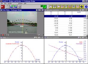
Let us describe briefly how the image measurement activity shown in the above screen dump goes. First of all, the activity allows collection of position data from the digital image. It is possible to place the origin of the coordinate system at any desired position and to rotate the axes, if necessary. You choose the correct scale by matching a ruler with a known distance in the image. Data are gathered by clicking on the location of points of interest. Data can be plotted and used for further analysis. In the lower-left window of Fig. 1, the regression tool has been used to find the quadratic function that fits the data best. In the lower-right window, you see the collected points once more, together with the data plot of the difference quotients (dy/dx) of consecutive points (plotted with respect to a second vertical axis). The difference quotients lie approximately on a straight line. The best line fit can be found with the regression tool. The third column of the table in the upper-right window also shows clearly the pattern for the difference quotients.
Mathematics of the Hanging Chain
Fig. 2 shows a screen dump of the activity in which the shape of a perfectly flexible chain hanging under gravity is investigated.
|
By collecting positions on the chain and trying a quadratic curve fit on the measured data, a pupil quickly finds out that the form of the chain is not a parabola (as Galilei erroneously claimed). At once, the simple question “How does a chain hang?” becomes a challenging problem. Pupils can follow in the footsteps of Huygens, Bernoulli, and Leibniz, who solved the problem of the catenary at the end of the 17th century, when differential calculus was discovered (Bos 1975). |
|
|
Fig. 2: Measuring and computing the shape of a hanging chain |
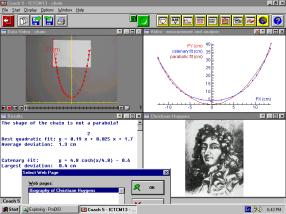
The function y(x) that describes the vertical position of a point on the chain as a function of the horizontal displacement x satisfies the following differential equation:
 ,
,
for some positive constant c. If the coordinate system is chosen such that the origin equals the lowest point of the chain, the solution is as follows:
 .
.
Of course, a pupil could try to match the data with this formula. But we prefer for our secondary school pupils a different approach to investigate the catenary.
We let the pupils study a similar, but simpler problem: “How does a chain with five objects of equal weight symmetrically attached hang under gravity?” The case of weights at equal horizontal distances is investigated first: the solution is a parabola. A screen dump of an important part of the activity is shown in Fig. 3. Measurements in the digital images reveal that the slopes of the right segments of the chain have a fixed ratio, viz., 1:3:5. Measuring in other images would convince pupils that this does not depend on the length of the segments or how far the suspension points are apart from each other. It turns out that one always has the following fixed ratio of positive slopes: 1:3:5:7:9:… Basic physics can explain this: equilibrium of forces holds at each point of application where a weight is attached. This simple observation allows computation of the shape of the system and it explains that the points of application are necessarily on a parabola.
|
|
|
|
|
|
Fig. 3: Measuring positions, angles, and slopes in a digital image |
|
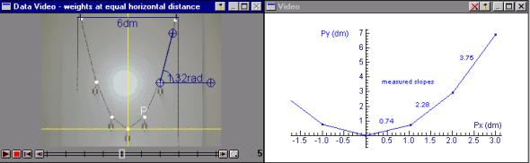
The next step is to realise that it also follows that the curve is not a parabola in case the weights are attached at equal distances along the chain. Finally, the fixed ratio can be utilised to approximate the free-hanging ‘ideal’ chain by modelling it as a string of 2n beads, for large n, where the beads are close at equal distance of each other.
|
When you choose a starting slope s0 between the lowest bead and its right neighbour, and when you keep the distance l between beads fixed, you can easily compute the position of subsequent beads, by realising that the slope increases with 2s0 at each step in the algorithm. Fig. 4 illustrates the use of the modelling environment of Coach for this purpose. Simulation runs with various values of s0 illustrate how the algorithm can produce a curve that fits the hanging chain. |
|
|
Fig. 4: Modelling the hanging chain |
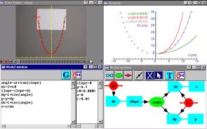
3 The classroom experiment
The profile of the 24 pupils of this research study has already been described at the end of the introduction. The practical assignment was not part of their examination portfolio, but it was graded as a regular test in the semester. The pupils work in pairs, mainly in a computer lab, and complete the assignment within two weeks. The estimated study load is 5 hours. The computer lab was reserved for them in the first week during their regular mathematics lessons (of 45 minutes) and on one afternoon. In the second week the pupils could make use of the computer facilities when available. After these two weeks, they had to hand in the report of their work (written with a text editor), a questionnaire, and a diskette with their Coach activities and results.
In our research experiment we wanted to get in particular answers to the following questions:
Do
the learning material and the chosen educational set-up enable pupils, who have
no prior practical experience with Coach, to acquire the right skills and
experience to use the data video tool effectively in their study of the shapes
of bridges and hanging chains?
Does
Coach, and in particular the data video tool, work without technical problems?
What
do pupils think of the software?
What
do pupils think of the subject, the learning material and of the use of real
data?
Since
it was the first time that pupils had to do practical work in the context of
mathematics, how do pupils like it and what difficulties did they encounter?
The tools used to get answers to these questions are classroom observations, video recordings (including video capturing of computer work), a questionnaire, and the reports of the pupils.
From the questionnaire we learn about the opinions of 8 teams. The pupils’ comments on Coach, in particular the video tool, and on the learning material are positive for the most part. Instructions about the use of Coach are clear and sufficient, so that it is easy to learn to use the video tool. Measuring angles and slopes in the computer environment causes no problems. Most pupils like the quick and easy way to measure on images and to display the data in graphs and/or tables. The 15 minutes demonstration of the learning environment at the beginning of the first activity starts is fine. The assignments link up well with each other and they do not take too long, as far as the collection of data for the report is concerned. All pupils find that theoretical part about the chain with 5 weights links up well with physics, but they differ in opinion about the mathematical background. Half of the pupils write that this part of the assignment does not link up well with their mathematical knowledge. In fact, many of them need assistance from the teacher.
Some pupils are a bit disappointed about the mathematical contents. They find that the assignments focus too much on learning Coach or on physics aspects, and that they less to do with mathematics. In retrospect, we must admit that they are right. We could have gone further into mathematical modelling[2] and we could have paid more attention to the role of symmetry, perspective, and the coordinate system in the problems. Especially the effect that a change of the coordinate system has on the data and on the formulas would have been an interesting topic and a natural introduction to the study of invariance of properties of curves under transformations. We also overlooked some opportunities while preparing the learning material. For example, to convince pupils that really more is needed than curve fitting for deep understanding of a shape, we could have asked them to apply the sinusoidal regression model
![]()
to the data collected for the Zeeburger bridge. They would have seen, maybe to their surprise, that this model works as good as the quadratic model. But which one is correct? And what do we mean by ‘correct’? Can a sinusoidal regression model approximate any piece of a parabola or are there limitations? Similarly, the pupils could have validated that the ‘ideal’ chain hanging under gravity with suspension points (-1,1) and (1,1), and with its minimum at (0,0) can be approximated very well by the rational formula
![]() .
.
What are actually the advantages of the exact formula for the catenary? Such tasks and question would have given the pupils more food for thought and they would have revealed the dangers of experimental mathematical modelling.
Most pupils like the practical work. For example, Jordi and Wester write: “It is more fun than the regular lessons, because the method is different from usual and more varied. Here you have to discover more by yourself.” Bianca and Alexandra comment as follows: “It is fun and it makes a change. It was not really difficult, not even the theoretical part. You must ‘see it’, and then it is easy. Please, do this more often.”
75% of the pupils write their report at home. Therefore, some of them indicate that they would like to have Coach available on their home computer. It turns out that we have been too cautious in our decision not to give the pupils the home version of Coach.
Do our classroom observations and the submitted reports confirm the positive reactions of the pupils? In general, the answer is yes. The enthusiasm of the pupils is great. Most pupils work without stops and we do not notice any negative attitude to work. They do their best to get accurate data in measurements. Pupils collaborate well: there are good discussions between teamworkers about what to do and how to interpret computer results, and fruitful discussions between teams that compare their results. Most teams work rather efficiently: one pupil reads the instructions aloud and the other pupil operates the personal computer. They switch roles many times so that both learn to use the learning environment. Occasionally this division of pupils’ roles causes confusion and problems, mainly because the pupil who operates the PC does not wait for complete instructions from his teammate, but goes ahead. Another problem that we notice is that pupils do not always continue reading where the stopped before and miss essential instructions.
The instructions to the pupils about reporting their work are deliberately very short: we want the pupils to think themselves about what and how to report about their activities. So, it is no surprise that reports vary much: some pupils just write down their results like tables and graph without much explanation, others give full report of activities, including their personal experiences. Although the pupils seem to be quite able to express themselves mathematically, it should be pointed out that they use of common mathematical notation. Otherwise they cannot resist the temptation of copying computer results without much questioning. We see in the pupils’ reports formulas like –7.2E-3x^2 + 0.69x + 28.16 and angles of 75.91º.
In the reports, the presence of units of length for slopes indicates that some pupils confuse slope and increase of a quantity. Maybe this is caused by the difference between mathematics, in which tangents are dimensionless, and science, where slope is treated as a quantity. Another interesting difference between the use of diagrams in mathematics and science pops up in the classroom experiment when pupils are making graphs invisible in a plot. To their surprise, pupils get weird diagrams with no coordinate system or no labels near the axes. They are thinking of a graph as a representation of a function, i.e., as a representation of a single object, so that it suffices to work with one variable. This is common in mathematics. In science however, a graph represents a relation between quantities. Then you must work with at least two variables.
Some pupils misunderstand the question in the third activity about the pattern in the angles and/or slopes of the chain segments. They write down that larger angle implies larger slope, and that the tangent of the angle is equal to the slope. They are right of course, but this was not the authors’ intention. Most pupils do not find the pattern from their collected data. They find the pattern first in the task to look at angles and slopes for the points (0,0), (1,1), (2,4), and (3,9) in the standard parabola y = x2, and then check if this also occurs in the measured data. This is not a wrong way of doing.
Let us end with possible extensions of the practical assignments. Firstly, pupils suggest the following subjects of practical work in which video and image measurement could play a role: the shape of the atrium at school, the streamline of cars, the supporting power of a structure, movements in sports, collisions, and acceleration, deceleration, and movements of objects. Many of them expect that it is more interesting and fun to work with video clips instead of with still images. We are of opinion that the discrete modelling approach offers an opening to the investigation of other systems of masses acting under gravity on a rope and that the scope of investigation can be broadened to anchor catenaries (Lamb 2000), shapes of suspension bridges, and to architectural structures. This kind of activities would illustrate the use of common mathematical shapes and functions such as straight lines, parabola, exponential and logarithmic curves, and it would reinforce some of the ideas of calculus. But more important, it would bring the real world into mathematics lessons in an attractive way.
Acknowledgements
This work was supported by a grant from the Netherlands Organisation for Scientific Research (NWO) in the programme “Teacher in Research”. We would like to thank the mathematics teacher Mr. Klein Entink at the Bonhoeffer College for allowing the experiment in his class. And last but not least, we thank the pupils for their enthusiasm at work.
References
Bos, H.J.M. (1975) The Calculus in the Eighteenth Century II: Techniques and Applications. The Open University Press.
Heck, A. (2000) Coach: an environment where mathematics meets science and technology. W. Maull and J. Sharp (eds.) Proc. ICTMT 4, Plymouth 1999. CD-ROM published by the Univ. of Plymouth,. http://www.tech.plymouth.ac.uk/maths/CTMHOME/ictmt4/P75_Heck.pdf
Beaufils, D. e.a. 1994) Images as a basis for computer modelling. Phys. Educ. 29, 89-93.
Escalda, L.T. and Zollman, D.A. (1997) An investigation o the effects of using interactive digital video in a physics classroom on student learning and attitudes. J. Res. Sci. Teach. 34 (5), 467-489.
Hilscher, H. (2000) Videoeinsatz in der Lehre. Physik in der Schule 38 (3): 193-200.
Lamb, J. (2000) Use only as much chain as you need. Practical BoatOwner 407, 117-119.
Laws, P. and Pfister, H. (1998)Digital Video Analysis in Introductory Mechanics Projects. The Physics Teacher 36,282-287.
Ministry of Education, Culture and Science (2000/2001) Secondary school. A guide for parents, guardians and pupils . URL: http://www.minocw.nl/english/doc/secondaryschoolguide.doc
Model of deformations of fluid particles
due to electric field
Iavor Varbanov Hristov
Sofia, Bulgaria
A mathematical model of finite deformations of compound drop containing another drop and two separate drops subjected to an electric field has been done. The fluids are homogenous, incompressible and Newtonian. The cases of concentric, eccentric and separate particles are investigated together.
1 Introduction
First studies in the field of deformations of fluid particles have been conducted by Taylor (1932). Later, Taylor (1934) has found critical velocity of shear flow, after which a drop set in the flow started to elongate. Taylor and Acrivos (1964) have proved that in uniform flow in Stokes approximation, an initially spherical particle remains spherical without any deformations. The problems of single drop set in viscous flow are prerequisite for solving the problems of compound drops (i.e. drop in drop), drop near to a plane wall or two separated drops. Brunn. and Roden (1985) have come to the conclusion that compound concentric drop set in uniform flow in Stokes approximation, as in the case of single drop, has shown no deformation. Chervenivanova and Zapryanov (1989) have observed that an eccentric compound drop in uniform flow in Stokes approximation shows deformations Using the Navier-Stokes equations and the finite element method, Bazlekov, Shopov, and Zapryanov (1995) have derived the finite deformations of an eccentric compound drop in uniform flow at middle values of Reynolds number. Sherwood (1988) has solved numerically the problem of fluid particle deformation under the influence of an electric field, using the boundary element method. By using the already obtained semi-analytical results for compound drop in a gravitational field, Sadhal and Oguz (1985) have come to the conclusion that the electric field in such problems can be used for stabilisation of different configurations (compound drop and bubble in drop), which is basis of the liquid membrane. The aim of this paper is to investigate the model of finite deformations of compound drop and two separate drops subjected to an electric field. The fluids at the three phases could be with different properties (viscosities, conductivities and permettivities), as the radii of the drops and the distance between them could have different values too.
2 Formulation of the problem
The problem for defining the finite deformations of a compound fluid drop subjected to an electric field is separated into two problems – electrostatic and hydrodynamic ones. By analogy with this problem, for defining the finite deformations of two separate drops subjected to an electric field we have the same formulation but with different boundary conditions.
|
|
|
|
|
|
Fig. 1: Scheme of compound drop subjected in an electric field |
|
In Fig. 1 the drop is two-component, compound of fluid 2 of viscosity m2, conductivity s2, permittivity e2 and fluid 3 of viscosity m3, conductivity s3, permittivity e3. The electric field that acts on the axis connecting the centres of the drops is with intensity Å0. It is causing the deformation of the two interfaces of compound drop. The initial form of compound fluid drop is spherical with undistorted radius R1 of the external sphere and undistorted radius R2 of the internal one. S1 is the interface between phase 1 and phase 2, and S2 is the interface between phase 2 and phase 3. The interfacial tensions over S1 and S2 are g1 and g2, respectively. The fluids 1, 2 and 3 are situated in W1, W2 and W3 respectively, while W1 is infinite area outside the drop.
The problem is solved in quasi-steady approximation, by using the reduced form of Maxwell equations (Laplace equations) and Stokes equations. The electric potential and the velocity are governed by the following equations:
|
|
Laplace equations |
|
(ê=1,2,3), |
(2.1) |
|
|
Continuity equations |
|
(i,k=1,2,3), |
(2.2) |
|
|
Stokes equations |
|
|
(2.3) |
|
|
|
|
where s is a stress tensor. |
|
The index k=1 when xÎW1, k=2 for xÎW2, and k=3 xÎW3, , while pk is the hydrodynamic pressure of the respective fluid. In the three phases, the electric potential jk, must satisfy the following boundary conditions
|
|
|
|
(2.1.a) |
|
|
|
|
(2.1.b) |
|
|
|
|
(2.1.c) |
|
|
|
|
(2.1.d) |
|
|
|
|
(2.1.e) |
where E0 is the intensity of the electric filed, X01 is x-component in Cartesian co-ordinate system Oxyz of the vector X0. s1, s2, s3 are the electric conductivity of the respective fluids and ¶/¶n is normal derivative to the surface, pointing to the respective domain.
The flow field must be governed by the following boundary conditions
|
|
|
|
(2.3.a) |
|
|
|
|
(2.3.b) |
|
|
|
|
(2.3.c) |
|
|
|
|
(2.3.d) |
|
|
|
|
(2.3.e) |
Here n is the unit normal vector at the interface S1 or S2, pointing out of the drops, while
|
|
|
|
|
is the Maxwell electric stress tensor for the respective phases (k=1,2,3), where ek is the electric permittivity of the different phases and Ek = - V jk. Let us assume that S1 and S2 are Lyapunov surfaces. The solution of (2.1) with boundary conditions (2.1.a-e) defines the electric potentials in all the three phases. The solution of (2.2, 2.3) with boundary conditions (2.3.a-e) gives the velocities in every point of S1 and S2. The deformation of the interfaces is determined by the normal component of the velocity and the kinematical condition
|
|
|
|
(2.4) |
Here XS is a point of the respective surfaces S1 or S2 and un is the normal component of the velocity at this point.
3 Results
The algorithm for obtaining the finite deformations of a compound drop and two drops subjected to an electric field was tested for a single drop in presence of an electric field and it was in compliance with the results of Sherwood (1988): Fig. 2 shows the deformation of single drop subjected to an electric field with the same parameters as Fig. 6 and the difference from Sherwood’s result is 3 %.
|
|
|
|
|
Fig. 2 |
Fig. 3 |
Fig. 4 |
On Fig. 3 is shown the deformation of two separate drops with the same properties as on the Fig. 3 from the experimental work (Zeks e.a. 1996). The difference between both results, theoretical and experimental, is less than 4 %. Fig. 4 shows the deformation of compound concentric drop, which compared with Fig. 6 (b) from Ha and Young (1999) has 2.5 % difference.
4 Conclusion
The problems of deformation of a compound liquid-liquid drop and two drops surrounded by a distinct third fluid in presence of an electric field are important for many fields of technology like industrial emulsions, biotechnologies, etc. In the present paper we show a model of the deformations of the fluid interfaces due to electric field. The results presented above show that the model has chosen appropriately, but there are properties of the fluid phases, for which the model doesn’t show good agreement with the experimental works. It’s caused by the numerical calculation error and by the reduction of the governing equations and the boundary conditions.
References
Bazhlekov, I., P. Shopov, Z. Zapryanov (1995) Unsteady Motion of A Type-a Compound Multiphase Drops at Moderate Reynolds Numbers. Journal of Colloid and Interface Science 169, 1.
Brunn, P., T. Roden (1985) On the Deformation and Drag of A Type a Multiple Drop at Low Reynolds Number. J. Fluid Mech. 160, 211.
Chervenivanova, E., Z. Zapryanov (1989) On the Deformation of Compound Multiphase Drops at Low Reynolds Number. Physico Chem. Hydrodyn 11, 3, 243-259.
Ha, J.W. and Yang, S. M. (1999) Fluid dynamics of a double emulsion droplet in an electric field. Phys. Fluids 11, No. 5.
Sadhal, S., Oguz, H. (1985) Stokes Flow Past Compound Multiphase Drops: The Case of Completely Engulfed Drops/Bubbles. J. Fluid. Mech., 160, 511.
Sherwood, J. D. (1988) Breakup of Fluid Droplets in Electric and Magnetic Fields. J. Fluid Mech, 188, 133-146.
Taylor, G. I. (1932) The Viscosity of a Fluid Containing Small Drops of Another Fluid. Proc. Roy. Soc. A 138, 41-48.
Taylor, G. I. (1934) The Formation of Emulsions in Definable Fields Flow. Proc. Roy. Soc. A 146, 501-523.
Taylor, T. D., A. Acrivos (1964) On the Deformation and Drag of a Falling Viscous Drop at Low Reynolds Number, J. Fluid Mech. 18, 466.
Zeks, B., Peterlin, P. and Svetina, S (1996) Chemical and Physical Effects on Red Blood Cells. Proc. 14th Int. Congress of Biometeorology Ljubljana, Slovenia.
Introducing models and modelling
through spreadsheets
Duncan A. Lawson and J. H. Tabor
Coventry, UK
2. Models from Next to Nothing
In applications focused mathematics degree courses there is an understandable desire to introduce students to the ideas and practice of mathematical modelling at an early stage. However, many mathematical models depend on a level of mathematical sophistication, such as differential equations, which most undergraduates do not have on entry to university. Furthermore, it is often the case with such models that specialist mathematical software is required for the solution of the model equations. This combination of sophisticated mathematics and unknown software can be a considerable deterrent to new undergraduates. This paper describes a way of introducing a range of key ideas within modelling, initially without using any new mathematical concepts, and relying on software which is both familiar and not specifically mathematical, namely the spreadsheet. A short description is given of a number of models which are easily explored with spreadsheets.
1 Introduction
Mathematical modelling is an integral part of any applications-based mathematics degree course. Many concepts within mathematical modelling are new to students starting out on their degree programmes. The majority of the mathematics that they have undertaken in their pre-university education has involved problems which have had a single correct answer (and often a ‘best' method for obtaining that answer). Many principles in mathematical modelling are alien to this culture. Often, there is not a correct answer and very rarely is there a single approach which can be guaranteed to produce an answer. It is therefore important to begin to introduce students to the ideas of mathematical modelling as soon as possible within their university studies.
Given that a key aim of this early introduction is to start the process of challenging the ideas of there always being a correct answer and a clearly defined route to obtaining it, it is important not to distract students by the mathematics that they must use in their modelling. This means that their initial experiences of modelling should be based in mathematics with which they are familiar. It also means that the situations they model should be ones which are easily understood and where the governing principles do not require detailed knowledge of another subject. In essence, the models should be based on situations which are everyday experiences or are governed by ‘common sense‘.
In practice, the majority of mathematical models used by professional mathematicians require the use of software to solve the model's governing equations. In some cases a purpose written program is required, in others a mathematical package may be sufficient. Requiring new students to learn to use such packages (or to write programs) will provide distractions from the key thrust of learning about modelling. For this reason models which can be investigated using only a spreadsheet make ideal introductory models. Although spreadsheets are capable of doing a wide range of mathematical tasks they are not specifically mathematical and, for most tasks, do not require knowledge of a considerable amount of syntax. Furthermore, in Great Britain, an increasing number of students are learning the rudiments of spreadsheet use in schools. This makes them much less likely to be deterred by using a spreadsheet in modelling than by using a mathematical package.
The combination of wanting to keep, initially at least, within the confines of familiar mathematics and software leads almost inevitably to discrete models. This immediately removes the need for any calculus. Although the students will have a knowledge of calculus, this is often less than complete and, in particular, their knowledge of differential equations will be limited. It might equally be said that they have no knowledge of methods for solving difference equations. However, the combination of discrete models and spreadsheet simulations is generally transparent. The spreadsheet simply carries out the calcuations required to generate the solution sequence. This transparency is not present in computer solutions of differential equations which, if algebraic, implement a mathematical solution method or, if numeric, use some kind of discretisation.
By using a carefully staged approach, starting in areas with which students are already familiar, it is possible to build up the ideas of modelling whilst introducing, almost incidentally, some new mathematical concepts. First session As discussed in the previous section, it is important to start with a situation where students are completely familiar with both the ‘laws' governing how things behave and also with the resulting mathematics. Money is something which most students know a good deal about and an introductory workshop based on individual sponsorship schemes has proved a valuable starting point.
Sponsorship Workshop
The students are told that a charitable organisation is willing to sponsor them through the first two years of their studies. The organisation is offering a choice of two schemes. In Scheme A the payment is £ 100 in the first month, increasing by £ 100 each month over the two years (so they receive £ 200 in the second month, £ 300 in the third month and so on). In Scheme B the payment is 1 penny (£ 0.01) in the first month and doubling every month (so they receive 2 pence in the second month, 4 pence in the third month and so on). Each student in the class is asked to write down which scheme they would choose. The majority usually choose Scheme A but some students will choose Scheme B. Their reasons for doing this vary. A few realise that the doubling process will eventually overtake the constant increase; whilst others make this choice because, although their intuition tells them that Scheme A should pay more, they regard this as too obvious and so choose the alternative.
The few students who have chosen Scheme B are then offered a revised version of Scheme A which pays £ 200 in the first month and increases by £ 200 each month. Any students who decline the revised scheme are offered progressively more money through Scheme A until only one student remains holding Scheme B. The students should then calculate how much, in total, they would be paid over the two years of their sponsorship to determine a ‘winner' from the group.
Although the totals can be calculated using the formulae for the summation of terms in arithmetic and geometric progressions it is better at this point to allow (or even insist) that students use a spreadsheet to perform the calculations. The students are then set the task of producing a spreadsheet which will allow them to calculate the total value of any revised scheme A by entering the value of a single parameter, the monthly increase (which is also the amount in the first month). The spreadsheet should also show graphs (on the same axes) of the growth of the running total of each scheme over the two year period. This spreadsheet can then be used to determine the value of the monthly increase which makes both schemes pay the same over the two years.
When everyone has established that this amount (to the nearest £ 10) is £ 560 they are then asked to estimate what the amount would have to be for the two schemes to pay the same if the length of the sponsorship period were three years rather than two. When this workshop was used with a group of new undegraduates at Coventry University on the first day of their course in October 2000 the estimates given ranged from £ 1000 to £ 5.6 million. One student did estimate that the amount should be £ 1 million. This is a remarkably good estimate as the correct value, to the nearest pound, is £ 1031824. However, the student's estimate may have been primarily based on selecting a large round number rather than out of a genuine feel for the specific size of the value.
Whilst it might be argued that there is little by way of modelling in this initial exercise it serves a number of useful purposes:
Students
gain practice in converting a problem into mathematics
They gain
experience in varying a parameter value to achieve a specific aim
They
revise their spreadsheet skills
They see
that Scheme A, with its constant monthly increase, grows steadily whilst Scheme
B, with its monthly doubling, grows very slowly for a considerable period of
time before a very rapid increase in the final stages
The last point is particularly important for the second session which does venture more into the world of modelling.
2 Models from Next to Nothing
The aim of the second session is to develop a model of the onset of vCJD. Before setting out the specifics of the model it is worth having a short class discussion about the way things grow and considering two specific ways:
1. Constant growth
This is illustrated by a machine that is producing items at the rate of c an hour. If xn is the number of items produced after n hours, it is clear that xn+1 = xn + c.
2. Proportionate growth
This is illustrated by an organism growing in such a way that every hour m new cells are produced per 1000 cells in the organism. If xn is the number of cells in the organism after n hours, it is clear that xn+1 = xn + m/1000 xn = r xn .
The spread of vCJD and its link with BSE in cattle is a current topic of interest across Europe. In the 80s BSE was a problem only in Britain but it is now an issue in many European countries. Although students will probably have little if any knowledge of what causes vCJD all they need is provided in a short article from the Sunday Times (Leake 2000). Broadly speaking, the key information may be summarised as follows:
1. vCJD is caused by the build up of abnormal prions in the brain (prions are formed from small proteins).
2. Normal prions are easily destroyed by the body's enzymes but abnormal prions are resistant to the body's defences.
3. Abnormal prions may be introduced to the body by eating infected meat.
4. The early victims of vCJD in Britain began to show symptoms approximately 10 years after being infected and died about 2 years later.
At first sight this does not appear to give sufficient information to develop a sensible mathematical model. However, it is in fact an excellent starting point. The development of the model illustrates the need to make reasonable assumptions and then to investigate the impact of these assumptions on the model.
To begin with we assume that symptoms will start to be displayed when the amount of abnormal prions in the brain reaches p % of the fatal amount. The students are asked to discuss between themselves what they feel is a reasonable value for p. The group of students referred to in the last section decided to take p to be 20.
The next stage is to produce a spreadsheet which implements both constant and proportionate growth models and to determine if either can represent the level reaching 20% after 10 years and 100% after 12 years. Students soon discover that the constant growth model is inappropriate whilst the proportionate growth model, with suitable choice of the growth rate parameter r can produce slow growth over the first 10 years followed by rapid growth. This reinforces what was learnt in the investigation of the sponsorships scheme in the first session. The monthly amount in scheme A displays constant growth, whilst in Scheme B there is proportionate growth.
The final product of this model is a spreadsheet which will predict the life expectancy of someone who has eaten a small amount of infected beef. Key parameters in this model are the growth rate parameter r (which is closely related to p) and the amount of infected beef eaten by the early victims of vCJD. The spreadsheet can be used to investigate the sensitivity of the model to these parameters, as described more fully in Lawson and Tabor (2001).
3 Linear models
It is a short step from the models
xn+1 = xn + c and xn+1 = r xn
to the linear model
xn+1 = a xn + b.
A practical situation leading to such a model, with which many students are familiar, is loan repayment. If we borrow £ A at a rate of interest of r % and make monthly repayments of £ P then, with £ xn being the amount still owed at the end of the nth year, we see that
xn+1 = ( 1+ r/100 ) xn - 12P with x0 = A
Once more a spreadsheet to perform the calculations is easily produced. The spreadsheet allows the user to input the values of A, r and P and then calculates the sequence of xn values. This can then be used to determine the monthly payments required to pay off the loan in a given period of time. The students should investigate the effect of A and r on the required monthly payments. There is a common tendency amongst students to think that most relationships are linear and this is reinforced by calling this a linear model. However, whilst the monthly repayments do depend linearly on A it soon becomes apparent that this is not true for r. Calculating the required repayments for any given amount with interest rates of 5% and 10% shows that the repayments do not double.
Whilst exploring linear models it is worth introducing a model where there are two variables. A model where the underlying assumptions are easy for students to understand and accept is the Richardson battle model. A simple description of this model is to let xn be the number of soldiers in one army at the start of the nth time period and yn be the number of soldiers in the opposing army. Then, assuming there are no reinforcements, we can postulate that
xn+1 = xn - a yn
yn+1 = yn - b xn
The number of soldiers in each army must decrease since some are being killed by the enemy. The assumption is that the number killed in one army is proportional to the number of soldiers in the other army. The two constants of proportionality (a and b) reflect the ‘efficiency' of each army which will depend on such things as how well trained and equipped they are.
Once more such a model is easily implemented in a spreadsheet. The important parameter values are a and b and the initial size of each army. An exercise which is accessible to most students is to use the Richardson model to represent the battle of Agincourt where 6000 British troops (mainly armed with longbows) defeated 30000 French and allied troops suffering only around 1000 casualties themselves. A slightly more difficult exercise is to model the Battle of Trafalgar, where the British fleet of 27 ships defeated the French fleet of 33 ships. At the end of the battle 18 French ships had been captured or destroyed whilst no British ship had been sunk (although some were damaged).
4 Data fitting
When the authors learnt to drive the Highway Code (Dept. of Transport 1969) contained a table giving the stopping distances for a car travelling at speeds from 20 mph to 70 mph. The stopping distances, in feet, were calculated from the formula v + v2/20, where v was the speed in mph. Giordano and Weir (1985) give data from experiments by the US Bureau of Public Roads which measured the actual stopping distances of a variety of cars with a variety of drivers. For each speed, the data give the range of stopping distances within which 85% of the measured values lie. At speeds up to 50mph the value from the British formula lies close to the middle of this range, but at higher speeds the British value drops towards the lower limit and at high speeds is below the lower limit. This suggests that, although the formula v + v2/20 contains simple coefficients which makes it memorable, it may not be the best to use over the range of speeds from 20mph to 70mph.
Students can be given the exercise of determining better coefficients in a formula of the form av+bv2. At this stage, this is purely an exercise in empirical modelling, the physics underlying the form of this formula can be discussed later if desired. This exercise forces students to address key questions such as ‘How do we judge whether one formula is better than another?' This allows discussion of different ways of measuring the error including maxmimum absolute error, summing absolute errors or error squares or using relative error measures. Students can initially be given some time to experiment with the effect of a and b on the chosen error measure before being introduced to the in-built routines which will find the ‘best' a and b for them (the Solver routines in Excel).
In line with the general trend to focus on the modelling no explanation need be given of how Solver works. However, if students have had some opportunity to experiment for themselves to try to find ‘good' values for a and b, they seem willing to believe that there is a systematic way of approaching the problem which simply requires a very large number of calculations to be made. They are therefore not disturbed by simply allowing the spreadsheet to do all the hard work for them!
This particular model is especially useful as the av term is easily interpreted and the value of the a coefficient can be used to determine the reaction time of drivers. The class can discuss whether this is a realistic value. Furthermore, once the ‘best' a and b have been found a plot of the errors across the data set shows a neat trend rather than random behaviour. This suggests the need for a more complex model. It transpires that a three parameter model of the form av+bv2+cv3 accurately represents the data and furthermore has a physical basis.
5 Population models
The limitations of proportionate growth in population models are easily shown for a bacteria colony. In the early stages the size of the colony grows in what seems a reasonable manner but after two weeks the mass of the colony is 4 tonnes and after 43 days it outweighs the earth. This leads to the need for a reduction in the per capita growth rate as the population increases and the discrete logistic model
xn+1 = xn + k (1 - xn / xM) xn
clearly has this property.
Once more this model is easy to implement in a spreadsheet. The key parameters here are the growth rate parameter k, the maximum sustainable population xM and the starting population x0 . The usefulness of the discrete logistic model can be illustrated by using the US population data from 1790 (this can be found in many places including Giordano and Weir 1985). This data has some excellent educational features. With appropriate values of k and xM the model shows excellent agreement with the data over the period 1790 - 1950. But then subsequent to this the model underpredicts the actual population. This allows discussion of the fact that parameters like xM cannot reasonably be taken to be constants for all time and that certain scientific discoveries may lead to the need to change their values from time to time. In the case of the US data the widespread use of anti-biotics which began around 1950 may be postulated to have increased the maximum sustainable population.
With the principles of intra-species competition established by exploration of the logisitic model for single populations it is now reasonably straightforward to extend to situations where different species interact. Conceptually the smallest extension is to competing species. In Britain there is a well-known example of this phenomenon: the usurping of the native red squirrel by the imported North American grey squirrel.
Working with a two species model of the form
gn+1 = gn + ( k1 - k3 rn - k5 gn) gn
rn+1 = rn + ( k2 - k4 gn - k6 rn) rn
as a general model of competing species (not just the grey/red squirrel competition) opens up new mathematical concepts such as equilibrium and stability. Once again the spreadsheet provides a means by which these ideas can be demonstrated visually as well as numerically without the need for sophisticated mathematical techniques. The idea of equilibrium points emerges naturally as, for a fixed set of ki values, the evolution of the g and r populations in time and in the GR plane are plotted. This can be used as a motivation to the simple algebra required to determine the location of equilibrium points without carrying out extensive calculations.
Stability can also be investigated from a calculational point of view. Once an equilibrium point has been located, the time development of the populations from initial values close to the equilibrium point are calculated using the same spreadsheet. The graphs may show the populations moving back towards the equilibrium point or moving away. Of course care is needed to ensure that a range of points close by are examined and also that the simulations are run for long enough for divergence to emerge. Whilst this is in no way a rigorous mathematical treatment it does serve the useful purpose of giving a convincing demonstration of the reality of instability in certain circumstances.
6 Conclusions
Spreadsheets are an ideal initial vehicle for investigating discrete models as they clearly produce the solution of the model equations by simply carrying out the required calculations. A sensibly constructed spreadsheet allows the effect and importance of model parameters to be easily explored. There are a range of models of phenomenon with which students are familiar and whose derivation require little specialist knowledge to understand and little advanced mathematics to analyse. These models are ideal for an introductory course as they allow students to focus on the modelling ideas and result interpretation without being distracted by the scientific or mathematical technicalities.
References
Department of Transport (1969) The Highway Code. HMSO, London.
Giordano, F.R. and Weir, M.D. (1985) A First Course in Mathematical Modelling. Brooks/Cole, Monterey, California.
Lawson, D.A. and Tabor, J.H. (2001a) Stopping distances: an excellent example of empirical modelling. Teaching Mathematics and Its Applications 20(2), 66-74.
Lawson, D.A. and Tabor, J.H. (2001b), APs, GPs and vCJD. Teaching Mathematics and Its Applications 20(1), 2-9.
Leake, J. Anatomy of a tragedy: how vCJD kills. Sunday Times, 5 March 2000.
Software Maple in teaching of ODE’s
Pavel Prazak and Antonin Slaby
Hradec Kralové, Czech Republic
The software Maple proved to be powerful assistant for solution various mathematical problems. It has efficient built in routines enabling wide variety of computations. It has also easy to use graphical commands to make visualization available. In our contribution we will focus on selected possibility of using symbolic calculations and graphical methods for illustration the subject of ordinary differential equations and outline various possibilities of visualization of the solutions of these equations and show the samples of application of above-mentioned problems.
At present computer technology belongs among the most rapidly developing areas of human activity. Its development highly influences also school system and educational process. Among vast areas of mathematics in which computer technology gives substantial help belong for example symbolic expressions, visualization of the solutions and the use of numerical methods. Maple belongs to the most powerful software products in above-mentioned areas. In our contribution we will show the use of this software packages for gaining solution of ordinary differential equation (ODE).
This package has several built in commands, which enable to avoid long and routine calculations. They enable to present and explain the explained subject matter in an innovative way. Last but not least they enable students to repeat and revise their knowledge of the taught chapters. Very important is the possibility to visualise the results and solutions using computer graphics. In connection with ODE we should mention graphical presentation of the solution ODE, direction line field of ODE, making graphs of isoclines, solution curves in the phase space. Graphical display enables students to understand better the meaning of obtained solution. Computer can provide a significant and quick help in this area and enables to solve also the problems, which could be performed only with a lot of difficulties otherwise.
1 Examples
We will restrict in further considerations to one first order differential equation or system of two first order differential equations. If we denote
|
|
|
|
our problem can be written in the following way
|
|
|
(1) |
|
|
|
|
As a solution of the equation we mean a function x = j(t), having a derivative on an interval I and fulfilling the following conditions
|
|
|
|
If there is in addition given the following initial condition
|
|
|
|
the problem is called Cauchy problem.
In case one ODE in (1) for each point [t, x] Î G function f has the only value x′(t). This number can be considered to be the direction (slope) of the line coming through the point [t, x]. Every segment having its middle point in the point [t, x], is called a linear element and a set of all linear elements is called direction line field of given equation. The sets of all the points for which holds x'=c or f(t, x) = c, c Î R are called isoclines.
|
Example 1: Let us consider the equation
Draw the direction line field and isoclines. The solution using software Maple is given in Fig. 1 including the commands needed. |
|
|
Fig.1: Direction line field and isoclines |
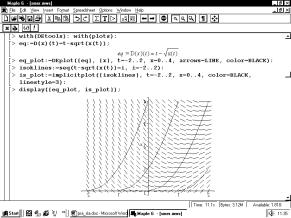
Example 2:
Braun (1983) describes the model of spreading technological information in a given industry branch. Let us suppose that the new technology is used by N0 firms at given amount of time t=0 and the number of all firms in branch let be N. Let us denote by N(t) the number of firms using new technology at time moment t. Let introduce the fraction
|
|
|
|
for further consideration, which specifies the rate of firms in this branch that use the new technology in a time moment t.
To simplify the model let us assume, that firms are willing to introduce the new technology only in case it is recommended for them by some firm using new technology. Then we can derive the following logistic equation
|
|
n'(t) = k n(t) [1-n(t)], |
|
where k is proportional constant. Let us presume for certainty that in a time moment t=0, the considered technology was in use by 1% firms in the branch and in time moment t=2 years the new technology has been used by 15 % firms. Find out the solution and plot the graph.
|
Using the following Maple commands > eq:=D(n)(t)=k*n(t)*(1-n(t)): > dsolve({eq}, {n(t)}); we obtain
with the constants k and C. As it is shown at Fig.2, these constants can be obtained as a solution of the system of equations following from the model. On this figure there are the rest steps of the solution. |
|
|||
|
Fig 2: The graph of solution of logistic equation |
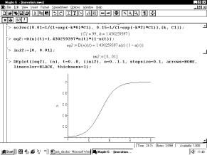
Let us investigate the exact equation
|
|
|
|
This equation has implicitly defined solution F(x, y) = c, c Î R. The set of points satisfying F(x, y) = c is called integral curve. Our next task is to demonstrate the way of displaying this curve. If we assume that there exists a parametric expression of this curve, then the exact equation can be transformed to the following system of two first order differential equations
|
|
|
|
By solving that system of equations we obtain parametric expression [x(t), y(t)] of integral curve F(x, y)=c, the arc of which is the graph of the solution of our exact differential equation. We will call the graph of the curve [x(t), y(t)] having the parameter t in the plane xy, in further text trajectory.
Example 3:
|
In a square
draw some integral curves of the equation -(cos x cos y)dx + sin x sin y dy = 0. Having with the help of Maple verified that we have really exact equation we can follow the procedure in Fig. 3. Let us remember the following notion that will be used in next problem. In the system (1) there is the so-called equilibrium solution x0, satisfying f(t,x0) = 0 for t Î I. |
|
|
Fig. 3: Integral curves of exact equation |
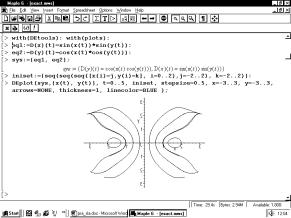
Example 4:
Phillips formulated a model in 1954 from which can be judged the time evolvement of production Y and investment I of certain macroeconomic unit (Allen, 1970). We will describe this model using two first order ODR.
|
|
|
|
where t denotes time, v investment coefficient, k and l speed of response, s marginal tendency to savings and A autonomous investments. Let
|
|
|
|
Let us display the trajectory of the solution, the functions I(t), Y(t) and the curve [t, Y(t), I(t)] for the problem having these initial conditions Y(0)=0, I(0)=0. Find in such a way the equilibrium solution. Having given constants and defined system of ODE, where we first equation denote eq1 and the second eq2, we can solve the system of equations.
|
>f1:=unapply(rhs(eq1), t): # right hand side of the equation eq1 becomes a function of t >f2:=unapply(rhs(eq2), t): >solve({f1(t)=0, f2(t)=0},{In(t), Y(t)}); In such a way we obtain the equilibrium solution In(t)=0, Y(t)=40, where In(t) denotes investments. By the command >DEplot({eq1, eq2}, {In, Y}, t=0..50, [In(0)=0, Y(0)=0], arrows=NONE, stepsize=0.25, thickness=1); |
|
|
Fig. 4: Trajectory of the system of equations in phase space |
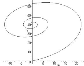
we obtain the trajectory shown on Fig. 4. If we omit the command arrows=NONE, then also the direction line field will be plotted.
|
By the commands >pl1:=DEplot({eq1, eq2}, {In, Y}, t=0..50, [In(0)=0, Y(0)=0], scene=[t, Y], stepsize=0.25, linestyle=3, thickness=1, linecolor=BLUE): >pl2:=DEplot({eq1, eq2}, {In, Y}, t=0..50, [In(0)=0, Y(0)=0], scene=[t, In], stepsize=0.25, thickness=1, linecolor=RED): >display({pl1, pl2}); we obtain the solution depended on time Y(t) and In(t) in Fig. 5. |
|
|
Fig. 5: Solutions Y(t) and In(t) |
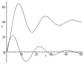
|
To get the idea of the whole graph of solution we can use the following command to obtain Fig. 6: >DEplot3d(({eq1, eq2}, {In, Y}, t=0..50, [In(0)=0, Y(0)=0], axes=normal, stepsize=0.25, thickness=1, linecolor=BLUE); The model we established by setting the constants k and l, possesses in our case decrement oscillating time behaviour. It means that both production and investments oscillate in macroeconomic system in time but there exist a steady state. |
|
|
Fig. 6: Specifying of the system of two first order ODR |
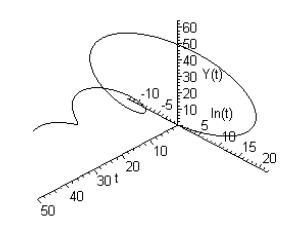
In addition to it from Fig. 5 there is certain that the production lags behind investments. If we set the constants in our problem differently we would obtain different time behaviour of solution and nothing prevent us from experimenting like this.
2 Conclusion
We could show only a few examples of using the software Maple for solution of ODE in our contribution. We claim to say that using Maple for teaching in this branch of mathematics is very motivated for our students of informatics. In spite of Maple being good assistant in learning of mathematics and solving various problems there also exist some disadvantages of this software package. Computer (software) isn't able to give always the right solution and consequently there keeps the task for teacher to show to students which solution (and in which way) responds to mathematical theory and its application and which solution is bad (or not possible to use).
References
Allen, R.G.D. (1970) Macro-Economic Theory, A Mathematical Treatment. Macmillan.
Braun, M. (1983) Differential Equations and Their Applications. Springer, Berlin.
Heal, K.M., Hansen, M.L., Rickard, K.M. ( 2000) Maple 6 Learning Guide. Maple Inc., Waterloo.
Milkova, E. (2000) Integration ICT into Educational Process. Modernizace vysokoskolske vyuky technickych predmetu. Gaudeamus, Hradec Kralove, 127 – 129.
Rab, M. (1995) Obycejne diferencialni rovnice. Masarykova Univerzita, Brno.
Turcani, M: (2000) Vyucba prirodovednych predmetov s vyuzitim ICT. ICTE Ostrava 2000. Zbornik.
Discrete delayed population models with Derive
Mazen Shahin
Dover, USA
1. Population models with first order difference equations
3. Controlling chaos in a system represented by first order difference equation
In this paper we show how Derive can be used efficiently in modeling and investigating discrete delayed population models. In particular we are interested in some population models represented by nonlinear second order difference equations. We will show how to generate a numerical solution of a given difference equation and investigate the stability of the equilibrium values of the system. We will apply an interesting and a practical method to control the chaos in a dynamical system represented by a single first order nonlinear difference equation. Some of the pedagogical issues related to the use of a CAS in modeling will be discussed.
1 Population models with first order difference equations
Let the population of a species at time n be denoted by Pn . Usually, the population one unit of time later, Pn + 1, is a function of Pn :
|
|
Pn + 1 = f (Pn) |
(1) |
A variety of f (Pn) has been used in different biological situations. A population of a species may be modeled by the first-order linear difference equation
|
|
Pn + 1 = (1 + a)Pn |
(2) |
where a is the unrestricted growth rate per period (e.g., year), and Pn is the population after n years. The solution of (2) is given by
|
|
Pn = (1 + a)n P0 |
(3) |
Equation (3) predicts exponential growth of the population, which is not realistic for most populations. Verhulst suggested in 1838 to replace equation (2) with
|
|
Pn + 1 = (1 + a)Pn - bPn2 |
(4) |
where b is very small positive constant compared to a, called the inhibiting constant. Equation (4) can be written in the form
|
|
Pn + 1 = rPn(1 - Pn / K) |
(5) |
Where K = r/b. Letting yn = bPn/r, equation (4) is scaled and transformed into the quadratic map (6),
|
|
yn + 1 = ryn(1 - yn) |
(6) |
where 0 < y0 < 1. Equation (5) shows that if Pn > K, then Pn+1 < 0, which is a drawback of this model. A more realistic and frequently used model is represented by
|
|
Pn + 1 = Pn exp[r(1 - Pn / K)], r > 0, K > 0 |
(7) |
Equation (7) can be scaled into (8) by letting yn = Pn/K, with the carrying capacity K = 1,
|
|
yn + 1 = yn exp[r(1- yn)], r > 0 |
(8) |
2 Discrete delayed models
In the above models it was assumed that every member of the species in the nth generation contributes to the population in the (n + 1)st generation. This assumption is true for certain species, such as most insects; however it is not the case for many other species where there is a substantial maturation period (e.g., 5-10 years for baleen whales), or species that migrate for breeding. Consequently the population model must incorporate a delay effect and is represented in the form
|
|
Pn + 1 = f (Pn, Pn - d) |
(9) |
One reasonable modification of equation (6) to incorporate the delay effect is (10),
|
|
yn + 1 = r yn(1 - yn - 1) |
(10) |
Equation (11) is a delay version of (8),
|
|
yn + 1 = yn exp[r(1 - yn - 1)], r > 0 |
(11) |
The International Whaling Commission (IWC) used equation (12) to model the baleen whale,
|
|
Pn + 1 = (1 - m)Pn + R(Pn - d) |
(12) |
where Pn is the adult population at year n and m is the death rate in any year with 0 < m < 1. In this model the adult population at year n + 1, Pn + 1, is the sum of surviving adult population from the previous year, (1 - m)Pn, and the adult population from births d years earlier, R(Pn - d). The factor R incorporates the unharvested equilibrium density, the per capita fecundity of females and the survival rate per year (see International Whaling Commission. Report No. 29. International Whaling Commission, Cambridge 1979).
Equations (10) and (11) are second-order nonlinear difference equations. Since, in general, there is no analytical solution of a nonlinear difference equation, we will use Derive to create numerical solutions in order to investigate these solutions. A numerical solution of a nonlinear second order difference equation can be found in different ways. One of these methods is to iterate the difference equation. Another method is to transform the second-order difference equation into a system of two first-order difference equations, and then investigate the system.
Let us find a numerical solution (n, yn), n = 0, 1, ..., 20 for the difference equation (10) with r = 1.25,
|
|
yn + 1 = 1.25 yn (1 - yn - 1) |
(13) |
with the initial condition y0 = 0.1 and y1 = 0.12. Since yn – 1 and yn are needed to compute yn + 1, we need to save yn - 1 and yn. Let us use y to represent yn - 1 and z to represent yn. We will use Derive’s function ITERATES as follows. Author the expression
|
|
A:= ITERATES([n+1, z, 1.25z(1 - y)], [n, y, z], [0, 0.1,0.12], 20) |
|
The approximation of this expression is the 3-column matrix [n, yn, yn+1]. To obtain [n, yn] we need to extract the first and second columns of the matrix A. This can be achieved by using Derive’s function EXTRACT_2_COLUMNS which is available in utility file ODE_APPRO.MTH. Load this file, author and simplify the expression
|
|
EXTRACT_2_COLUMNS(A, 1, 2) |
|
Now we can graph yn vs. n.
Equilibrium values and stability
To find the equilibrium values (fixed points), E, of a second order difference equation, substitute E for yn+1, yn, yn - 1 and solve for E. For example the difference equation (10) has two equilibrium values E = 0, and E = 1 - 1/r. The equilibrium value E = 0 has no biological meaning, since it indicates that the population Pn = 0. Consequently equation (13) has the equilibrium values E = 0 and E = 0.2. There are different methods to determine the stability of an equilibrium value of a difference equation.
Method 1 - Graphical analysis:
One of these methods uses an intuitive definition of stability. This method is employed by creating numerical solutions of the difference equation with initial conditions close to the equilibrium value. Create a numerical solution with initial condition(s) less than the equilibrium value and another numerical solution with initial condition(s) greater than the equilibrium value. The equilibrium value is
stable
if both solutions converge to the equilibrium value,
unstable
if both solutions diverge from the equilibrium value,
semistable
if one solution converges to the equilibrium value and the other solution
diverges from the equilibrium value.
For example, to study the stability of the equilibrium value E = 0.2, students create the numerical solutions of (13) with initial conditions less than 0.2, e.g., y0 = 0.18 and y1 = 0.16; and with initial conditions greater than 0.2, e.g., y0 = 0.25 and y1 = 0.3. It is easy from the graphs to conclude that the equilibrium value E = 0.2 is stable.
Method 2 - Linearization about the equilibrium value:
Let us use equation (13) to illustrate this method. To study the stability for E = 0.2, we linearize the difference equation (13) about E = 0.2, by letting
|
|
yn = en + 0.2 |
(14) |
where en represents the difference between yn and the equilibrium value 0.2 (the error from equilibrium). Using equation (14), equation (13) reduces to
|
|
en + 1 = - 1.25 en en - 1 + en - 0.25 en – 1 |
|
If we choose y0 close to 0.2, e0 will be close to 0 and the quantity e0 e1 can be neglected compared to e0 and e1. Thus, the approximating difference equation is
|
|
en + 1 = en - 0.25 en - 1 |
(15) |
which is a second-order linear difference equation with constant coefficients. Now we can use Derive=s function LIN2_CCF in the utility file RECUREQN.MTH to find the solution of (15). Recall that the function LIN2_CCF(p, q, r, n, c1, c2) computes the general solution of the second-order difference equation (16) in terms of two constants c1 and c2,
|
|
yn + 2 + pyn + 1 + qyn = rn |
(16) |
where p and q are constants and rn may be a function in n. Now to find the solution, en, of (15) author and simplify the expression LIN2_CCF(- 1, 0.25, 0, n, c1, c2), which gives
|
|
e - 0.693147 n (c1 + n c2) |
(17) |
The limit of (17) for n®¥ is 0, that is lim n®¥ en = 0. This means that the solutions yn®0.2 as n®¥. Consequently, the equilibrium value E = 0.2 is stable.
Similarly the linearization of the nonlinear difference equation (10) around the equilibrium value E = 1 - 1/r produces the linear equation (18),
|
|
en + 1 - en - (1 - r)en - 1 = 0 |
(18) |
The solution of (18) is
|
|
yn = ( r - 1)0.5n [ c2 COS(n ATAN (4r - 5)2 ) + c1 SIN (n ATAN (4r -5)2 )] |
(19) |
Using Derive to evaluate lim n®¥ yn for different values of the parameter r helps students to determine the long-term behavior of the solutions.
3 Controlling chaos in a system represented by first order difference equation
It is well known that the solutions of the quadratic map (6) for values of r Î (3.5699, 4] do not approach a fixed point or periodic cycles and behave erratically. In addition they are very sensitive to the initial conditions. This type of behavior is called chaotic. There are some methods to control chaotic systems. Guemez and Matias (J. Guemez and M. A. Matias, Control of Chaos in Unidimensional Maps, Phys. Lett. A 181 (1993), 39 - 32) suggested an interesting and simple method to control deterministic chaos of a system represented by a first order single difference equation. The method works by applying a series of proportional feedbacks (adjustments) on the system variable performed periodically with a certain period. The method, like some other methods, stabilizes a given unstable periodic orbit. However the method is simpler (more robust) than other methods since it does not require detailed information about the system and it does not change system parameters.
Let us rewrite equation (6) in the form
|
|
yn + 1 = 4λyn (1 - yn) |
(20) |
Guemez and Matias= control algorithm consists of the application every Δn iterations of a feedback to the variable yn (the population size) having the form
|
|
yn = yn (1 + γ) |
(21) |
where γ is a real number represents the strength of the feedback, and - 1 < γ < 1. Let Δn be some positive integer representing the period of control. Then every Δn we change the population size at the beginning of that generation yn by yn (1 + γ). Note that in this case n is a multiple of Δn. Thus the control is given by
|
|
|
{ |
4λyn (1 - yn) |
if n does not divide Δn |
|
|
|
yn + 1 = |
|
|
(22) |
|
|
|
|
4λyn (1 - yn) |
if n divides Δn |
|
We will show how Derive can be used to apply Guemez and Matias control method to the system modeled by equation (20) for selected values of the parameters λ, γ, and Δn. Similarly we apply this method to the system modeled by (8).
[1] Newer versions of Coach will indeed contain a data image tool because it offers more possibilities to users.
[2] As a matter of fact, we have done a practical assignment about mathematical modelling of parabola and the catenary in a class of pupils in their second year of upper education. It was a success and one pupil commented that this was one of the few times that she was forced without mercy to think deeply. The English translation of this project can be downloaded from the web page www.science.uva.nl/~heck/research/quadmod