Strand 5:
Cooperation between
Dynamic Geometry Software and
Computer Algebra Systems
Martín Garbayo Moreno
Madrid, Spain
|
Plenary lecture: |
Boosting the geometrical possibilities of Dynamic Geometry Systems and Computer Algebra Systems through cooperation |
|
A study of conics with Maple V and Cabri-Géomètre II |
|
|
The three and four bar linkages revisited: Graphs and equations |
|
|
A computer aided learning environment of linear algebra using the computer algebra system MuPAD |
|
|
Bridging the gap between dynamic geometry and computer algebra: The case of loci discovery |
In this strand, a new investigation area was opened as a result of the logic process of integration of both systems, CAS and DGS, which had hardly interact for the moment. Having both systems grown enough, in the same way as in Mathematics History, the obvious process was to put the Abstract Algebra (not empiric) in touch with the Synthetic Geometry. In the plenary session, Eugenio Roanes gave a wide overview of the current available software, and, after stating that there have been some approaches in the direction marked in the strand title, he insisted on the pseudo-empiric treatment in the approaches of proof implemented in packages such as Cinderella or Cabri-Geomètre. He indicated those research directions, which should guide the collaboration between the CAS and DGS systems, using automatic proofs; in the way it is being carried out nowadays using Groebner basis.
The talk presented by Yuriko Baldin is an elegant integration of conics representation in the plane using their definitions as geometric places and their graphical representation as the intersection of a cone and a plane. As she points out, the separate visions given to the students make difficult to integrate both definitions of a conic. If Cabri is used in the plane and Maple in 3D, she shows that both visions of the conics can be presented simultaneously. Notice also that it caused great expectation the representation in real time of the intersection of cones and planes, and it lead to discussions in some other talks, which considered these real time representations not to be available.
Both papers presented by José Valcarce and Francisco Botana gave a solution very similar to the one proposed by Roanes in the plenary session. Both had designed their own application of Dynamic Geometry related with Algebra. In one of the talks they illustrated how their application Locus worked, showing, after having carried out the graphical representation of a geometric place, how their package gave the equation of that place. In the other talk, they treated problems with singularities are still present, and how they solve them. In this presentation, an interesting discussion took place treating that certain singularities were not still solved; this discussion went on after the lecture.
Finally, the talk given by Wolfgang Fraunholz and Frank Postel was divided into two parts. On the one hand, the package MuPad was shown as a very useful tool to teach some concept to the students. It resulted very interesting the introduction and the example, which showed how this kernel application could be used to develop particular applications. The example gave a very clear idea of the huge potentiality and usefulness of this MuPad option.
We regret enormously the absence of Susana Carreira: she proposed a very interesting talk.
Last, but not least, we would like to thank the conference staff for their kindness and their great concern for solving every incident each time we ask for help.
Dear Hermann and Manfred, we will forget neither Klagenfurt nor its surroundings after the reception you gave us.
Boosting the geometrical possibilities of Dynamic Geometry Systems and Computer Algebra Systems through cooperation
Eugenio Roanes-Lozano
Madrid, Spain
1. Introduction and state of the art
2. Is isolated evolution possible?
3. Evolution in collaboration: Filling the existing gap
5. Possibilities of the implementation
Both Computer Algebra Systems (CASs) and Dynamic Geometry Systems (DGSs) have reached a high level of development, but, unfortunately, they have evolved independently. Some CASs (like Maple) include specific and powerful packages devoted to Euclidean Geometry, but no CAS has incorporated mouse-drawing capabilities. Moreover, no tools have been provided to fill the gap between the well-known DGSs and the usual CASs in order to have the possibility to draw a geometric configuration with the mouse, and to obtain the equations of the drawn configuration. This is made possible by the package described below. To obtain complicated formulae from sketches, automatic theorem proving and automatic discovery are examples of straightforward applications.
1 Introduction and state of the art
Computer Algebra Systems (CASs), like Maple, Derive Mathematica, Axiom[1], Macsyma, Reduce, MuPad [2] see the list of web sites at the end for more information) ... are specialized in algebraic calculations. They use exact arithmetic and can handle non-assigned variables (i.e. variables in the mathematical sense, not in the usual sense in Computer Science). Many extensions like symbolic differentiation and integration, linear and non-linear equation and polynomial system solving, 2D and 3D plotting... are usually included too. There are some specific purpose-ones, like the excellent (and free)
CoCoA, specialized in computing Gröbner bases in polynomial fields over finite characteristic fields[3].
Dynamic Geometry Systems (DGSs), like The Geometer's Sketchpad, Cabri Geometry II, Cinderella, Euklid, Dr. Geo, WinGeom, Autograph, The Geometric Supposer ... (see also the list of web sites) are specialized in rule and compass Geometry. The adjective dynamic comes from the fact that, once a construction is finished, the first objects drawn (points) can be dragged and dropped with the mouse, subsequently changing the whole construction. They usually incorporate animation and tracing too. As far as I know, Cinderella is the only one that offers the possibility to deal with non-Euclidean Geometries. Moreover, it is the only one that keeps background calculations in  (what avoids the drawing from vanishing in exceptional cases). Unfortunately, CASs and DGSs have evolved independently. Some CASs (like Maple) include specific and powerful packages devoted to Euclidean Geometry. Some authors have also developed geometric packages for other CASs, like Derive (Kutzler 1996). But no CAS has incorporated Dynamic Geometry capabilities. The need for cooperation is, as many other key ideas, already underlined in the book Recio (1998; unfortunately available only in Spanish). This lack of cooperation is more surprising in cases like the TI-92 calculator from Texas Instruments -
http://education.ti.com/us/product/tech/92p/features/features.html
- where both technologies are simultaneously available. On the other hand, Dynamic Geometry Systems can't handle (at least from the point of view of the user) non-assigned variables. Therefore, what can be saved from a DGS is only a live graphic (to be read by that and only that DGS), a geometric algorithm (script or macro, to be interpreted by the DGS) or a dead (fixed) graphic in one of the standard graphic formats. It looks like a certain software product (The Algebraic Geometer, from Saltire Software -
- will offer this possibility. This product has been announced for some time, but is not on sale yet. Exactly at the interval between beginning to write this article and its deadline, some Spanish researchers (J.L. Valcarce and F. Botana) have implemented in visual-Prolog an impressive DGS named Lugares (Valcarce and Botana 2001). Now at a beta-version level, this DGS can communicate with CoCoA, can produce automatic proofs of geometrical theorems (see Cox e.a. 1992, Chou 1988, Kreuzer and Robbiano 2000, Roanes-M. and Roanes-L 1994, Roanes-L and Roanes-M. 1996 a, b, Wen-Tsun 1984a, b) and can even complete geometrical theorems (it can sometimes found missing hypotheses for a theorem to become true), i.e., perform automatic discovery Recio and Vélez 1999, Roanes-M. and Roanes-L 2001) Moreover, The Geometer's Sketchpad will possibly offer the possibility to export parametric code to CAS in the release following v.4.0 (v.4.0 is now at a beta-level). We'll detail all these ideas, already sketched in Roanes-L and Roanes-M. 2000), afterwards.
2 Is isolated evolution possible?
Can a CAS evolve isolated to fulfil these requirements?
To complete a CAS with mouse-driven geometrical capabilities as a user seems impossible. Not to say about dynamic capabilities. Moreover, I don't think any developers’ team would be interested in implementing such an extension.
Can a DGS evolve isolated to fulfil these requirements?
Only to make the DGS handle non-assigned variables and work in exact arithmetic seems impossible as a user. For a developers team it should mean e.g. to start again from the beginning in exact arithmetic...
3 Evolution in collaboration: Filling the existing gap
What would be needed from the DGS?
To be precise, what would be needed from the DGS is only the possibility to handle and export parametric data about the plot: coordinates of points (allowing parameters as coordinates), equations of objects (allowing parameters as coefficients), length of objects (depending on parameters)...
Example 1: If A Î R2 is the intersection of axes x and y, its coordinates are (0,0). The coordinates of a point B Î R2 lying on the x-axis can be, at a certain moment t0, (2,0), but its parametric (general) coordinates are (b1,0) ; b1 Î R. Similarly, if C Î R 2 is a free point, its coordinates are, in general, (c1,c2); c1, c2 Î R, although at moment t0 they can be e.g. (3,5). Then the parametric equation of line BC is
c2 × (x - b1) - (c1- b1) × y = 0
(to which the parametric point (c1,c2) clearly belongs), despite the fact that at moment t0 it can be
5x – y – 10 = 0
(to which point (3,5) clearly belongs).
What would this allow?
This relatively small change would allow exciting new possibilities like:
i) to sketch with the DGS a parameter-dependent geometrical construction and to obtain its exact equations. These equations could be used for any process (like writing an exam in a word processor, obtaining conditions for a locus, trying to manually produce a step by step proof of a theorem with a CAS...)
ii) to directly perform the whole process of automatic theorem proving automatic discovery beginning just with geometrical sketches [4] and through the automatic call from the DGS to the CAS, that works hidden in the background.
The latest development in DGS
A possibility would be to switch from the existing DGS to one of the emerging and newly designed DGS or to wait for the classic DGS to develop these possibilities. In fact, Lugares is able to fulfil task ii) of the previous subsection. As it is treated in another article in this book, we shall not get into detail here. The commercial version of Lugares and possibly the version following release 4 of The Geometer's Sketchpad will incorporate possibility i) as an enhancement.
Analysing how the gap can be filled (in cooperation)
Let us analyse how the right extensions for the existing software could be developed in order the CAS and the DGS to cooperate. Initially I think there are four ways to do it:
I From inside the DGS: Normally the source code of the DGS is not available to the user. Therefore this approach requires the cooperation of the designers of the DGS. As said above, this author suggested the designers of The Geometer's Sketchpad to try to provide parametric equations of objects in the release following v.4. Nevertheless this approach shouldn't be too hard (for the developers of the DGS!), as internally the system has to maintain a hierarchy of objects not based on actual (numeric) but on some kind of parametric coordinates. This need was also suggested by this author to the developers of Lugares, where it is straightforward, as it is already able to send these data to CoCoA.
II From the DGS as a user: We have unsuccessfully tried to develop a tool that provides such parametric equations from the new constructor named tool of The Geometer's Sketchpad 4 beta-version (in fact we can construct the parametric equation of the first level children objects, based on the parents objects parameters, but the nature of these objects is not recognized by the system, so the construction can't go deeper than one step, what is almost useless). This was the closest we got to our goal. We didn't succeed with any other DGS either.
III From the CAS: A first idea would be to use the numerical equations provided by the DGS. But this soon becomes inoperative, as after a few steps and given only the numerical equations, it is almost impossible to obtain the parametric equations.
IV Using the geometric algorithms of the DGS: The DGS are also able to define general step-by-step constructions (scripts in The Geometer's Sketchpad v.1 to v.3, the description in the .html in The Geometer's Sketchpad v.4, macros in Cabri-Geometry, Construction Texts in Cinderella...). And these are nothing but geometric algorithms! These geometric algorithms (sequences of geometric elementary constructions and operations) could then be translated (using a translator designed ad-hoc) into sequences of algebraic equations and algebraic operations that could be used by the CAS.
The idea developed afterwards is to analyse and develop approach 4.
4 The package
We shall refer hereafter to The Geometer's Sketchpad 3.0 (1995) and Maple 6.01 (Char e.a. 1991a and b, Heck 1996, Corless 1995, Roanes-M. and Roanes-L 1999 for which these pieces of software were developed.
The Geometer's Sketchpad was chosen because it is really friendly (specially its scripts). Maple was chosen because it is also very friendly and its Gröbner bases package is very powerful and well documented. Nevertheless the implementation could be developed for different (and crossed) DGS and CAS.
The Geometer's Sketchpad's scripts: Exporting the construction
The Geometer's Sketchpad can save both figures (denoted sketches) and geometric algorithms (denoted scripts). Scripts can be saved in The Geometer's Sketchpad's internal format for scripts or in readable format (.TXT).
Example 2: For instance, let us consider the script generated by the construction of the circumcircle of a triangle (that, once defined, is able to automatically construct the circumcircle of any triangle, given its vertices).
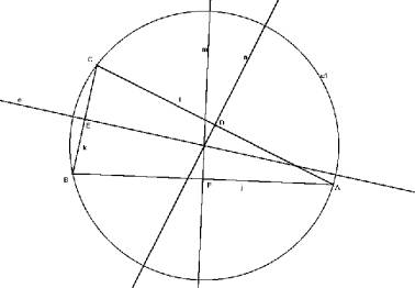
Fig. 1: Sketch of the construction of the circumcentre of a triangle
If saved in text mode, looks like
Script01.gss
Given:
Point A
Point B
Point C
---------------
Steps:
1. Let [j]=Segment between Point A and Point B.
2. Let [k]=Segment between Point B and Point C.
3. Let [l]=Segment between Point C and Point A.
4. Let [D]=Midpoint of Segment [l].
5. Let [E]=Midpoint of Segment [k].
6. Let [F]=Midpoint of Segment [j].
7. Let [m]=Perpendicular to Segment [j] through Midpoint [F].
8. Let [n]=Perpendicular to Segment [l] through Midpoint [D].
9. Let [o]=Perpendicular to Segment [k] through Midpoint [E].
10. Let [G]=Intersection of Line [o] and Line [n].
11. Let [c1]=Circle with centre at Point [G] passing through Point A.
what looks pretty close to mathematical standard language. Now it should be transformed into a Maple-like appearance.
Translator from scripts to Maple-acceptable syntax
An external translator, relatively similar to Pareja and Roanes-L. (1989), was initially developed in Logo language (WinLogo 1991a, b, H. Abelson 1982; Logo was chosen due to its facilities to deal with lists). This was abandoned in favour of another complete translator written in Maple by Carl Devore (Newark University).
The idea is that the user only has to introduce the parameters of the so called given points. Maple will perform the subsequent calculations (that the DGS presented in geometric form) in algebraic form.
Example 3: If the input is the listing in the previous subsection, the output will be:
#Given: point(A,A_x,A_y);
point(B,B_x,B_y);
point(C,C_x,C_y);
#---------------
#Steps:
segment(j,A,B);
segment(k,B,C);
segment(l,C,A);
midpoint(D,l);
midpoint(E,k);
midpoint(F,J);
perpendicular(m,j,F);
perpendicular(n,l,D);
perpendicular(o,k,E);
intersection(G,n,o);
circumCP(c1,G,A);
To obtain it, the user would only have to
 start a Maple session
load the paramGeo
Geometry package
load the Sketchpad-to-Maple
translator
execute the translator applied
to the .TXT of the script corresponding to the drawing
(optional) give a
particularization of the coordinates of the given points, e.g. A_x:=1; A_y:=0;
read the .MPL
translation of the .TXT (it is automatically executed line by line when read).
Afterwards, all the coordinates, equations... of the objects in the sketch will be available to the user (in Maple).
The lacks of Maple's geometry package
Maple 6 already incorporates an excellent geometric package (named Geometry). Unfortunately (and surprisingly), this package can't handle parameters (i.e., for example coordinates of points that define a line should all be numerical).
Example 4: Let us transcribe what happens:
> with (geometry):
> unprotect(D): #D is a reserved word in Maple
> point(C,[0,0]):
> point(D,[2,3]):
> line(r,[C,D]):
> Equation(r);
> enter name of the horizontal axis> x;
> enter name of the vertical axis> y;
-3 x + 2 y = 0
works. But, the similar
> point(A,[a1,a2]):
> point(B,[b1,b2]):
> line(s,[A,B]):
geometry/checkline: One of the following conditions must be satisfied -b1 <> 0 -b2 <> 0
Error, (in geometry/checkline) not enough information: the line is not defined
clearly fails.
ParamGeo: A ''Parametric Geometry'' package for Maple
ParamGeo, the ''Parametric Geometry'' Maple package developed by the author, is very similar to Maple's standard Geometry package. Nevertheless, it presents the following advantages
i) it is designed to directly translate The Geometer's Sketchpad constructive steps
ii) parametric coordinates can be given to the initial points and it can deal with these parameters along the subsequent calculations.
A first version of this package was presented at ACA'2001 Conference (31st May-3rd June 2001, Albuquerque, NM, USA) and it has been greatly improved.
The procedures implemented are:
Declarative procedures: point, line, segment, circumference by
centre and point, circumference by centre and radius
Constructive procedures: midpoint, parallel line, perpendicular
line, intersection of two algebraic sets of points (intersection)
Boolean procedure: point membership (isIn)
Auxiliary procedure: distance
Derived procedures: perpendicular bisector, angle bisector.
Membership declarative procedure: point is on object.
Let us describe them:
point
input: a name and two
coordinates.
job: assigns [5] to the name the list of the two coordinates .
line
input: a name and two
names of points.
job: assigns to the name the equation of the line through those two
points.
segment
input: a name and two
names of points.
job: assigns to the name a list formed by the equation of the line
through those two points and the two names of points.
CircumCP
input: a name and two
names of points.
job: assigns to the name the equation of the circumference with centre
in the first point, through the second point.
CircumCR
input: a name, a name of
point, a name of segment.
job: assigns to the name the equation of the circumference with centre
in the first point and radius the given segment.
Midpoint
input: a name and the
name of a segment.
job: assigns to the name the list of the two coordinates of the midpoint
of the given segment.
Parallel
input: a name, the name
of a segment or line, the name of a point.
job: assigns to the name the equation of the parallel line to the given
line or segment through the given point.
Perpendicular
input: a name, the name
of a segment or line, the name of a point.
job: assigns to the name the equation of the perpendicular line to the
given line or segment through the given point.
Intersection
input: a name and
exactly two names [6] of algebraic sets (lines or circumferences).
job: it returns either “No solution” or “Unique solution” (and assigns
to the name the coordinates of the point) or ''Two solutions'' (and assigns to
the name, followed by ''1'', the coordinates of one of the intersection points
and to the name, followed by ''2'', the coordinates of the other intersection
point).
IsIn
input: the name of a
point and the name of an object from {line, circumference}.
job: it checks whether the given point is in the given object, returning
True or False accordingly.
Dist
input: two names of
points.
job: it returns the distance between the two points (in exact
arithmetic).
PerpBis
input: a name and a name
of segment. [7]
job: it assigns to the name the equation of the perpendicular bisector
of the given segment.
AngleBis
input: a name and three
names of points.
job: it assigns to the name the equation of the angle bisector of the
angle of vertex the second point and which ray-sides pass through the first and
third points, respectively.
PointOnObject
input: the name of a
point, the name of its x-coordinate and its y-coordinate, and a
name of algebraic object.
job: it adds to the list of added relationships, LREL, the
polynomial obtained by substituting in the polynomial defining the algebraic
object all the ocurrences of x and y by the x-coordinate and y-coordinate of the given
point, respectively. [8]
All procedures are simple from the mathematical point of view, but in some of them several different cases have to be taken into account to return the equation the usual way (e.g. line) or to consider all possibilities (e.g. intersection). Others, like circumCR are straightforward. For the sake of brevity the code is not included, but circumCR is included as an illustration afterwards.
circumCR:=proc(c_,P_,r_)
local p1_,p2_;
p1_:=op(1,P_);
p2_:=op(2,P_);
assign(eval(c_),
(x-p1_)^2+(y-p2_)^2-r_^2=0);
end:
Example 5: If Maple is ordered to perform the calculations at the end of Example 3 (G is the intersection point of perpendicular bisectors o and n) and
> G;
is typed afterwards, then
2 2
1 1 -C_x + C_x + C_y
[ - , - -------------------- ]
2 2 C_y
is obtained. Those are the coordinates of the circumcentre, G, of triangle ABC.
Remark: The Geometer's Sketchpad automatically assigns letters to objects. To avoid conflicts with Maple's reserved letters, objects denoted D, O, I, x, y are renamed D_, O_, I_, x_, y_ by the translator, respectively.
5 Possibilities of the implementation
Sketching geometric constructions
As seen in Example 5, the coordinates of the circumcentre have been obtained without typing a single equation.
Automatic theorem proving in geometry
Although normally the process is not so simple, let us include a trivial example, needing to use neither Gröbner bases method nor Wu's pseudoremainder method. Let us check that point G of Example 5 lies in the third perpendicular bisector.
>m;
1
x - - = 0
2
>isIn(G,m);
true
and that it is really the cirumcenter of the triangle, i.e., that its distances to A, B and C are equal.
>simplify(dist(G,A)-dist(G,B));
0
>simplify(dist(G,A)-dist(G,C));
0
Applications in education
A straightforward application of this cooperation would be to treat with the computer the whole mathematical process of discovery (or re-discovery):
Investigating ® Guessing ® Checking ® Proving .
DGS Lugares can already perform the whole process (it directly produces the proof). But with the possibility described in the first section of chapter 3, the last step could be performed and controlled by the student.
Acknowledgments
This paper is partially supported by project TIC2000-1368-C03-03 (Ministry of Science and Technology, Spain).
Many people have helped directly or indirectly in making this work possible. In alphabetical order:
Francisco Botana (Universidad de Vigo), for providing a beta version of the impressive new DGS Lugares, and an interesting e-mail correspondence regarding these problems
Carl Devore (Newark University), who implemented directly in Maple a very smart ''Sketchpad-to-Maple'' translator that substituted for good the initial external translator
John Olive (Georgia University), who introduced DGS to me several years ago and with whom I discussed for several hours about this paper at Atlanta, and which expertise in The Geometer's Sketchpad made it possible to produced a tool for the new release 4 beta that partially covered my needs
Steven Rasmussen (Key Curriculum Press), for kindly providing a sample copy of the friendly El Geómetría, Spanish version of The Geometer's Sketchpad
Tomás Recio (Universidad de Cantabria), that possibly introduced automatic theorem proving in Geometry in Spain, leads a line of research in automatic discovery, and that indirectly or directly (like in this case) influences so many research works in Mathematics
Eugenio Roanes-Macías (Universidad Complutense de Madrid), for his tireless interest in automatic theorem proving in Geometry, and his comments and suggestions that improved this paper
Scott Steketee (Key Curriculum Press) for his kindness and patience when discussing the details of a possible future enhancement of The Geometer's Sketchpad.
6 Conclusions
Algebra is possibly the most powerful language for Geometry, meanwhile DGS and CAS have evolved isolated from each other.
It has been shown along the paper how some new DGS are presenting or will present a new feature: the possibility to cooperate with a CAS for different tasks (among them automatic theorem proving and automatic discovery).
An analysis of this cooperation and how it could be developed for existing DGS and CAS has been detailed.
I think it is a most interesting cooperation that can boost the possibilities of both kind of systems.
List of sites for software
http://www.autograph-math.com/
http://www.cet.ac.il/math-international/first.htm
www.education.ti.com/product/software/cabri/features/features.html
www.education.ti.com/product/software/derive/features/features.html
www.education.ti.com/product/tech/92/features/features.html
www.keypress.com/catalog/products/software/Prod_GSP.html
http://math.exeter.edu/rparris/
www.zib.de/Optimization/Software/Reduce/address_reduce.html
References
Abelson, H.(1982) IBM Logo. Byte Books/McGraw-Hill.
Buchberger, B. (1988) Applications of Gröbner Bases in non-linear Computational Geometry. Rice, J.R. (ed.) Mathematical Aspects of Scientific Software. Springer, 59-87.
Char, B.W. e.a.(1991a) Maple V Language Reference Manual. Springer.
Char, B.W. e.a.(1991b) Maple V Language Library Reference Manual. Springer-Verlag.
Chou, S.C. (1988) Mechanical Geometry Theorem Proving. Reidel.
Corless, R.M. (1999) Essential Maple. Springer.
Cox D., Little, J., and O'Shea, D. (1992) Ideals, varieties, and algorithms. Springer.
Heck, A.(1996) Introduction to Maple. Springer
Kortenkamp, U. (1999) Foundations of Dynamic Geometry (PhD. Thesis), Swiss Fed. Inst. Tech. Zürich.
Kreuzer, M. and Robbiano, L. (2000) Computational Commutative Algebra. Springer-Verlag.
Kutzler, B. (ed.)(1996) Introduction to DERIVE for Windows (Chapter 12).
Pareja, C. and Roanes-L., E. (1989) Traductor Automático Logo Inglés-Logo Español. Publicaciones Pablo Montesino, Universidad Complutense de Madrid.
Recio, T. (1998) Cálculo Simbólico y Geométrico. Ed . Síntesis.
Recio, T. and Vélez, M.P. (1999) Automatic Discovery of Theorems in Elementary Geometry. Journal of Automated Reasoning 23, 63-82.
Roanes-L., E. and Roanes-M., E. (1996a) Automatic Theorem Proving in Elementary Geometry with DERIVE 3. The International DERIVE Journal 3(2), 67-82.
Roanes-L., E. and Roanes-M., E. (1996b) Mechanical Theorem Proving in Geometry with DERIVE-3. Barzel, B. (editor): Teaching Mathematics with Derive and the TI-92. ZKL-Texte Nr.2 , 404-419.
Roanes-L., E. and Roanes-M., E. (2000) How Dynamic Geometry could Complement Computer Algebra Systems (Linking Investigations in Geometry to Automated Theorem Proving). Proc. of the Fourth Int. Derive/TI-89/TI-92 Conference, Liverpool 2000. Published in CD-ROM by BK-Teachware.
Roanes-M., E. and Roanes-L. E. (1994) Nuevas Tecnologías en Geometría. Editorial Complutense, Madrid.
Roanes-M., E. and Roanes-L., E. (1999) Cálculos Matemáticos con Maple V.5. Ed. Rubiños.
Roanes-M., E. and Roanes-L., E. (2001) Automatic Determination of geometric loci. 3D-extension of Simson-Steiner Theorem. Campbell, J and Roanes-L., E. (eds.): Proc. of AISC'2000. Springer, LNCS 1930, 157-173.
The Geometer's Sketchpad (1995) User Guide and Reference Manual v.3. Key Curriculum Press.
Valcarce, J.L. and Botana, F. (2001) Lugares. Manual de Referencia. Universidad de Vigo.
Wen-Tsun, Wu (1984a) On the decision problem and the mechanization of theorem-proving in elementary Geometry. A.M.S. Contemporary Mathematics 29, 213-234.
Wen-Tsun, Wu (1984b) Some recent advances in Mechanical Theorem-Proving of Geometries. A.M.S. Contemporary Mathematics 29, 235-242.
WinLogo (1991a) Guía de Referencia. Idea, Investigación y Desarrollo.
WinLogo (1991b). Manual del usuario. Idea, Investigación y Desarrollo.
A study of conics
with Maple V and Cabri-Géomètre II
Yuriko Yamamoto Baldin and Yolanda Kioko Saito Furuya
São Carlos, Brazil
4. Activities with Cabri and Maple
In this work we present a study of conics using Maple V and Cabri-Géomètre II aiming an integration of bi and tri-dimensional approaches to this subject. The usual presentation of conics in elementary instruction is based on the plane geometry, starting from focal properties and then making a connection of geometry to algebra, by means of quadratic expressions. This approach hardly explains the geometric meaning of the eccentricity or of the directrix lines. On the other hand, with the 3-dimensional approach, in which conics are presented as plane sections of a symmetric cone, the fundamental focal properties of conics are quite hard to be seen and understood. Usually, the two approaches seem to be taught as separate topics. Nevertheless, the most beautiful applications of conics to real-world problems, which motivate the teaching of this topic at elementary/secondary schools, demand the conics to be recognized in 3-dimensional settings. We present a study with combined use of CAS (Maple V) and DGS (Cabri-Géomètre) which integrates both approaches in the classrooms, turning the teaching of this fascinating subject more complete and meaningful. We include useful exercises on Dandelin constructions with Maple V and Cabri-Géomètre, which help the teacher to construct concrete teaching material on the subject.
1 Introduction
The use of technology in the classrooms has brought many changes to teaching practices, and one of most remarkable facilities is the possibility of visualization of geometric objects, which leads to a better understanding of geometric properties and applications. Yet, the traditional way of teaching conics is grounded on the plane geometry, starting from focal properties within the framework of analytic geometry, making then connection of geometry to algebra of quadratic expressions.
The dynamic interaction with geometric objects, available in DGS like Cabri-Géomètre II, brings new perspectives to teaching / learning process of conics with plane geometry, either analytic or purely geometric points of view.
The plotting facility of CAS like Maple V permits easily the visualization of conics as plane sections of a (symmetric) cone, which are actually their origins and much explored since the Greeks. The animation feature is very handy to explore the different types of degenerate and non-degenerate conics.
In this work we use Maple V and Cabri-Géomètre II as software tools, indicated shortly as Maple and Cabri.
The main motivation to our work is the fact that we realize the progressive domination of plane analytic point of view in the instruction of conics in secondary schools (in Brazil), and somehow students and teachers are forgetting the 3-dimensional treatment. Frequently, the study of conics as space curves is restricted to a simple presentation of their nomenclature and does not explore the connection to their basic properties. A better knowledge on conics will lead naturally to beautiful applications of this topic in real-life problems such as mirrors, telescopes, astronomy, etc. In this paper we propose classes with simultaneous use of Maple and Cabri to make the integration of 2 and 3- dimensional aspects of conics. The activities were tested during a course for prospective teachers at Universidade Federal de São Carlos, Brazil, in 2000.
2 First step
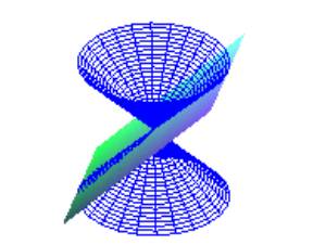
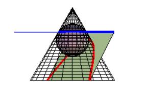
We propose an introduction to the subject “conic” starting with a Maple presentation of a two-fold rotational cone, and different possibilities of its intersection with a plane are explored. Manipulating the plot in order to visualize the effects from different points of space is very didactical. If the class is more advanced, the teacher can try to explain the use of either implicit form or parametric form of representation of a surface. The exploration of degenerate and non-degenerate conics and their classification using animation of planes is very easy, and constitutes an example of what can be done better with technology than in traditional classes. Fig. 1 illustrates a Maple presentation of a parabola as a plane section of a symmetric cone. The plane is animated so that the degenerate curve of parabolic type is easily observed. Also, the slope of the intersecting plane respect to a generator of the cone can be related to this situation, with the facility of manipulation of plots of Maple.
|
|
|
|
Fig. 1: Degenerate conic of parabolic type and a parabolic section |
|
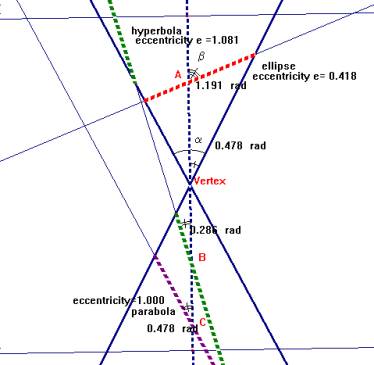
When we visualize the conics as different types of plane sections, we can introduce the concept of profile plane as a plane, which contains the axis of rotation of the cone. The intersection of a profile plane with the cone produces a 2-dimensional setting that makes it possible the study of the classification of conics through its profile, using Cabri. This procedure of reducing 3-dimensional setting into plane geometric situation is clearly useful to modeling and solving 3-dimensional problems. The eccentricity of conics can be introduced at this time, comparing the 3-dimensional and 2-dimensional illustrations.
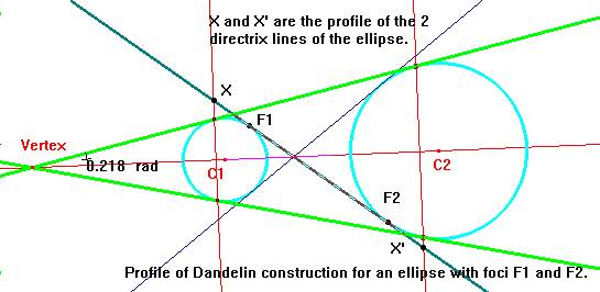
Fig. 2 illustrates a study with Cabri of the eccentricity of a conic related to the slope of intersecting plane that originates the section, as e = cosine (b)/cosine (a), where a is the half-angle of the vertex of the cone and b is the acute angle between the axis of the cone and the intersecting plane.
|
|
|
|
|
Fig. 2: Eccentricity and the conics in a profile plane |
||
The manipulation of geometric data yields a dynamic interaction with the plot, which facilitates the understanding of the connection between 2-dimensional and 3-dimensional treatment of conics, including the degenerate cases. Observe also that the dynamical experimentation on this plot shows a circle as a limiting case of an ellipse.
The method of studying conics as sections of a two-fold cone is due to Greek mathematician Appolonius of Perga (260-190 BC). Actually, the teacher may recall that the nomenclature of non-degenerate conics comes after Appolonius, and is traditionally related to the slope of the intersecting plane referred to the axis of the cone. In Boyer (1968) we find the real ideas of Appolonius for the nomenclature of conics, as well as other characterizations of conics before Appolonius. In this paper we are not going to present these ideas, although it is quite interesting to explore these early conceptions of conics and relate them to the known properties. We remark that the use of technology largely contributes to facilitate this study, which we consider as a nice opportunity to use the History of Mathematics as teaching strategy.
The traditional teaching of conics usually follows from this point to plane geometry, beginning with the characterization of non-degenerate conics as plane geometric loci satisfying well-defined focal properties, and then the analytic geometry is introduced to connect the conics to algebra of quadratic expressions. Cabri has very appropriate tools to study many constructions of conics as loci, as well as to deduce analytical expressions. In Baldin-Hasegawa-Villagra (2001) and Jennings (1994) there are nice applications of conics to classroom activities, which lead to interdisciplinary instruction with physics. With 3-dimensional geometric presentation as done so far, the fundamental properties of conics studied with analytical tools are not evident, and we believe that this is a turning point for teachers to make a difference in the development of their classes on this topic.
3 Dandelin constructions
The geometric constructions (1822) due to the Belgian mathematician G. P. Dandelin provide a nice way to discover the focal properties of the conics given as space curves contained in a cone (Jennings 1994). It is very helpful to have at hand a didactical kit of Dandelin constructions, made with some transparent material for the cone in order to visualize the inscribed spheres that are tangent to a conic section. These models can be seen in good Museums of Science around the world (like in Boston, MA, USA or in Milan, Italy) but it is not usual to find them in Brazilian secondary schools. Therefore the teacher is challenged to build the models by him (her) self.
This task brings forth some problems, which turn to be interesting problems of geometry. The first of such problems are:
“Given a sphere and an outside point at a fixed distance from its
center what is the vertex angle of a single folded symmetric cone with the
vertex at the given point in which the sphere is inscribed?” (for a parabola).
“Given two spheres of different diameters and a fixed distance
between their centers, what is the vertex angle of a single folded symmetric
cone in which the spheres are inscribed?”
(for an ellipse).
“Given two spheres and a fixed distance between their centers, what
is the vertex angle of a two folded symmetric cone in which the spheres are
inscribed in different halves?” (for a hyperbola).
The limitations of sizes of sphere models available in stationary stores and the difficulty in planning the actual making of the Dandelin models faced by our students have motivated the use of Maple and Cabri as either a visual teaching aid or a guide to the construction of the didactical kit
4 Activities with Cabri and Maple
The reduction of the problem to plane geometry by means of a profile of the cone and the respective non-degenerate conic suggests the use of Cabri with the ruler and compass methodology. This is very good exercise of plane geometry and the problems stated above are respectively equivalent to the following:
“Given a segment r1 and points C ¹ V with r1 > dist(V,C) what is the angle between the line VC and a line by
V that is tangent to the circle with
radius r1 and center C?”
“Given two segments r1 ¹ r2 and two points C1 and
C2 far apart by a fixed distance
d ³
r1 + r2, what is the angle
between the external tangent lines to
the circles with respectively center Ci and radius ri, i = 1,2?”
“Given two segments r1 and r2, and two points C1 and C2 far
apart by a fixed distance d > r1 + r2, what is the angle between the
internal tangent lines to the circles with respectively center Ci and radius ri, i = 1,2?”
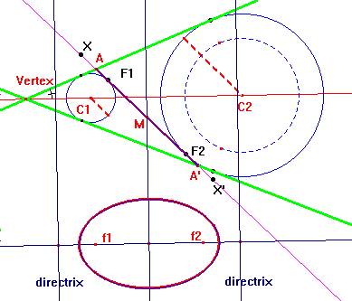
Constructing and combining appropriate macro-constructions of Cabri for the solutions to these problems we get nice solutions of the problems of Dandelin constructions, with the localization of the foci and the profile points of directrix lines in each case. The manipulation of the data allows an interesting study of the data-dependence of the solution, in each case. Also the construction in the same file of the conic curve obtained using the data from the profile plane shows the connection of geometric concepts as eccentricity and directrix lines in the plane of the curve with those introduced in 3-dimensional setting.
On the other hand, the 3-dimensional visualization of Maple is a wonderful teaching aid to really understand the principles of Dandelin constructions, but to produce the desired output one has to first realize and solve the geometric data using analytical and algebraic tools, based on the same arguments used in Cabri solution. Then the Maple solution is obtained programming the geometric data, which turns this solution more difficult to execute than Cabri, at least for secondary level students and teachers.
The advantage of Cabri solution is based on its purely geometric arguments that are actually very didactical, and the advantage of Maple is the visualization of real models with the possibility of understanding the position of the foci and the directrix lines for each non-degenerate conic.
Fig. 3 illustrates a profile of an elliptical section of a cone with Cabri, and Fig. 4 shows the corresponding ellipse in the plane.
|
|
|
|
|
Fig. 3 |
||
|
|
|
|
|
Fig. 4: An ellipse in the plane with its profile in the cone |
||
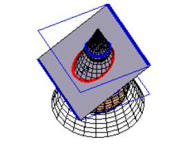
The following figures were obtained with Maple, programming the geometrical data.
|
|
|
|
Fig. 5: Dandelin model for a hyperbola |
|
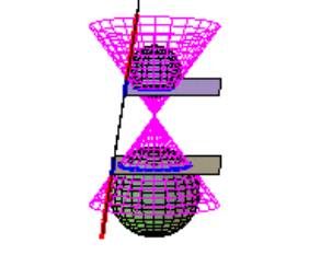
We can observe the directrix lines and the foci. The manipulation of 3-dimensional plot is quite interesting and very didactical.
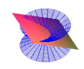
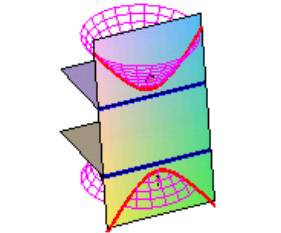
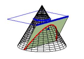
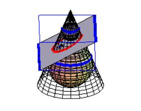
Fig. 6 and 7 are Maple solutions to Dandelin Models for Parabola and Ellipse.
|
|
|
|
Fig. 6: Dandelin model for a parabola |
|
|
|
|
|
Fig. 7: Dandelin model for an ellipse |
|
We omit the details of the programming with Maple as well as the corresponding figures with Cabri for Hyperbola and Parabola.
5 Conclusion
The limitation of the pages does not allow including more examples of the combined use of Cabri and Maple in classroom activities for conics, recovering the geometrical aspects of this subject. For example, other problem that can be solved using Cabri and Maple in the similar context is:
“Given a cone and a plane, find the radii of Dandelin spheres which fit to the different positions of the plane respect to the axis of the cone”.
Also it is very interesting to study other characterizations of conic sections such as those previous to Appolonius or those using oblique cones.
The files containing the mathematical details of the study presented in this paper for both Cabri and Maple are going to be accessible in English version at the site:
http://www2.dm.ufscar.br/~atividades/conicas/.
We expect that this study would bring the attention to the helpful collaboration between CAS and DGS that contributes to filling the gap between 2-dimensional and 3-dimensional approaches in teaching geometry and to making a connection of mathematics to real-world applications through a meaningful teaching mathematics with technology. See Baldin e.a. (2001) for some application.
References
Baldin, Y.Y., Hasegawa, R.T. and Villagra, G.A.L. (2001) Focal properties of conics and applications. Proceedings of 2nd Cabriworld. Montréal. To appear.
Boyer, C.B.(1968) A History of Mathematics. J. Wiley.
Jennings, G.A. (1994) Modern Geometry with Applications, Universitext. Springer.
The three and four bar linkages revisited: Graphs and equations
Francisco Botana and José L. Valcarce
Pontevedra, Santiago, Spain
2. Loci in current dynamic geometry systems
3. A symbolic approach to loci generation
This paper reviews the behaviour of current dynamic geometry systems (The Geometer’s Sketchpad, Cabri Géomètre, Cinderella, Geometry Expert and Lugares) when dealing with a simple linkage: the three (or four) bar linkage. The different approaches to numerical generation of loci are discussed, highlighting their success and limitations. Dynamic linkage generation can be used in engineering education and real design, overcoming the need of books for designers.
1 Introduction
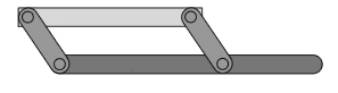
A four-bar linkage, illustrated in Fig. 1, is one of the simplest mechanisms. A chain of four links is the minimum basis for a useful mechanism. Although it is frequently called-named a three bar linkage, a true three link chain makes useless machinery.
|
|
|
|
|
|
Fig. 1: A four bar linkage |
|
There are many specialized computer programs suited for the study and design of these linkages among other mechanisms, but we will focus on the capabilities of current dynamic geometry environments to cope with them. In this way, we show how this software can be efficiently used in basic mechanical engineering teaching.
The steps for constructing a four bar linkage in a dynamic geometry environment can be summarized as follows:
1. Draw a circle with centre A and fixed radius.
2. Add a point B on this circle and draw the segment AB.
3. Draw a circle with centre C and fixed radius, not intersecting the first circle.
4. Draw a circle with centre B intersecting the circle cantered at C.
5. Take one of the intersection points of these circles, D, and draw BD and DC.
The link AC, not usually drawn in these systems, is called the foundation link, AB is the input or driver link, DC is the output or driven link, and BD is the connecting link. Fig. 2 shows the construction of a four bar linkage in Lugares (Valcarce and Botana 2001).
|
|
|
|
|
|
Fig. 2: A four bar linkage in Lugares |
|
2 Loci in current dynamic geometry systems
A common way to test the behaviour of the linkage in these environments consists of obtaining the locus of the midpoint of the connecting link. So, we construct the midpoint M of segment BD and select this point and B (the order of selection depends on the chosen system). The standard facility for drawing loci in dynamic geometry systems allows us to get the locus of the midpoint. Fig. 3 shows (in the usual order of reading) the obtained locus in five systems: The Geometer’s Sketchpad, GSP, (Jackiw 1997), Cabri Geometry (Laborde and Bellemain 1998), Cinderella (Richter-Gebert and Kortenkamp 1999), Geometry Expert, GEX (Gao e.a. 1998), and Lugares (Valcarce and Botana 2001).
|
|
|
||
|
|
|
|
|
|
Fig. 3: The locus of the midpoint of the connecting link in five DG systems |
|||
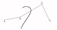
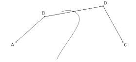
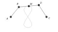
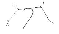
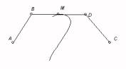
It is well known the way that these systems use to generate the locus: B can move only along the circle cantered at A, so the driver link rotates with B. The constraints imposed to the mechanism and the trace of the connecting link midpoint give a sequence of points in the screen. A simple linear interpolation, with predefined number of samples, is used to produce the locus line. The reason behind the different loci produced by Cinderella and the others is as follows: The last step to construct the linkage assumes that the circles cantered at C and B intersect, using one of the intersection points to define the links BD and DC. When B moves along the first circle, it can happen that those circles do no intersect anymore, therefore disappearing the whole linkage. Is this behaviour, geometrically correct and plausible in this virtual environment, reasonable in a material setting? The linkage would not stop when AB and BD are perpendicular, but it would move backwards, guided by the other intersection point D’ (Fig. 4).
|
|
|
|
|
Fig. 4: The true locus of the midpoint |
||
While the classical approach to loci needs both intersection points to produce the whole locus, Cinderella detects the moment when D runs into complex space, changing immediately the direction in which B traverses the circle. Its treatment of continuity causes that the remaining half locus will be obtained.
3 A symbolic approach to loci generation
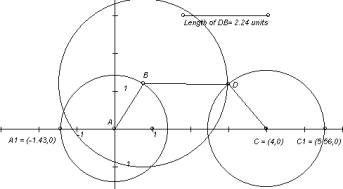
Apart from having the standard loci generation, Lugares incorporates an interface to communicate with a computer algebra software (Valcarce and Botana 2002). The system can export an algebraic translation of the geometric construction. In our case, the linkage consists of a set of points and properties, shown in Figure 5.
|
|
|
|
|
Fig. 5: The Discover window in Lugares |
||
We find the locus of the midpoint M constructing a free point and declaring it to be such a point. Using the Groebner basis algorithm (Buchberger 1985, Recio 1998), in a similar way to Macías and Locano (1999), Lugares returns the equation of the locus, as shown in Fig. 6 .
|
|
|
|
|
Fig. 6: The locus equation |
||
Furthermore, Lugares can plot the curve equation (Fig. 7).
|
|
|
|
|
Fig. 7: The graph of the locus line in Lugares |
||
4 Conclusions
We have reviewed the three bar linkage generation in current dynamic geometry environments. It is shown that in most systems the loci of some link points is not complete. The symbolic approach of Lugares allows its whole generation, as in Cinderella, returning also the loci equation.
References
Buchberger, B. (1985) Groebner bases: an algorithmic method in polynomial ideal theory. Bose, N.K. (ed.) Multidimensional Systems Theory. D. Reidel Publishing Company, Dordrecht, 184-232.
Gao, X.S., Zhang, J. Z., Chou, S. C. (1998) Geometry Expert. Nine Chapters Publ., Taiwan.
Jackiw, N.(1997) The Geometer’s Sketchpad. Key Curriculum Press, Berkeley.
Laborde, J. M., Bellemain, F. (1998) Cabri Geometry II. Texas Instruments, Dallas.
Recio, T. (1998) Cálculo simbólico y geométrico. Síntesis, Madrid (in Spanish).
Richter-Gebert, J., Kortenkamp, U. (1999) The Interactive Geometry Software Cinderella. Springer, Berlin.
Roanes Macías, E., Roanes Lozano, E. (1999) Búsqueda automática de lugares geométricos. Boletín de la Soc. “Puig Adam” de Prof. de Matemáticas-Congreso IMACS-ACA’99, 53, 67-77.
Valcarce, J. L., Botana, F. (2002) Bridging the Gap between Dynamic Geometry and Computer Algebra: The Case of Loci Discovery. Proc. ICTMT 5. Klagenfurt 2001.
Valcarce, J. L., Botana, F. (2001) Lugares. Manual de Referencia. Technical Rep., Univ. Vigo, Pontevedra
A computer aided learning environment
of linear algebra using
the computer algebra system MuPAD
Wolfgang Fraunholz
Koblenz, Germany
The aim of this learning programme is to help students to get acquainted with the elements of linear algebra. Two levels are provided:
the secondary school level
the university level for newcomers (especially those who need linear
algebra as a tool for other subjects, i. e. engineering science, physics,
economics and others)
|
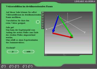
In the first level the content is taught, which is usually taught in German grammar schools, in the second level the content of linear algebra within a lecture on mathematics for scientists, for engineers or for economists. See the table of content at http://euler.uni-koblenz.de/inhaltla The subjects of the first level are condensed in the first chapter, named vectors. The other chapters contain the well-known subjects of elementary linear algebra. The speciality of this programme is the use of the computer algebra system MuPAD, which had been developed by the MuPAD-group of Prof. Fuchssteiner at the university of Paderborn and was represented in the talk of Frank Postel (see there). This CAS makes available two controls: the calc control and the graph control, which can be used for arithmetic problems respectively for geometric problems preferably in three dimensions. How these controls are integrated in the learning environment can be seen on Figures 1 and 2. |
|
|
|
Important for the learner is the interactivity to cope with a task, with a problem by himself or herself. Therefore there will be a lot of exercises, which will be constructed bottom-up, so for instance:
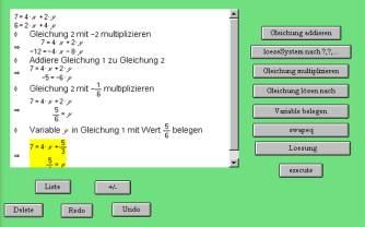
If the Gauss-Jordan-elimination is to be done, at first the students have to do it step by step and they only get the command buttons for
multiplying a row by a number
adding one row to another
changing two rows
So initially they cannot use a command like “do the Gauss elimination” or “do Gauss-Jordan”. Later on – e. g. when calculating determinants – they will have commands like “Gauss elimination” to get a diagonal matrix, so that they can multiply the diagonal elements to get the value of the determinant. But again they have not the command “determinant”, which will be used later on in the course. So the students should learn at first the procedure, e. g. solving a system of linear equations, doing elementary row operations of a matrix or calculate the value of a determinant. Finally the students should have learned the most important topics of linear algebra and be able to use a computer algebra system solving the problems within linear algebra.
Some of the educational aims are
To get the concept of the vector, of vector algebra, of matrices, of
determinants, of eigenvectors and so on
To improve the knowledge of the three-dimensional topology
To give an impression of application of concepts of linear algebra
The following examples will point up these aims:
|
1 |
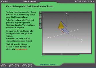
Translations in the 3-dimensional space: - Three-dimensional topology. A cone will be moved by a parallel displacement. The students may rotate the axis in two degrees of freedom in order to watch the cone and the trans-lasting arrows, which represent a vector. So they should get the concept of the vector as a class of arrows of the same length and the same direction. |
|
|
2 |
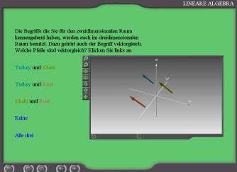
Equality of vectors - concept of vector: The task is to find out if two or three arrows represent the same vector. Again the students can rotate the figure to compare the given arrows. Repeating the exercise they get at random new arrows. So they will also practise the perception of the three-dimensional space. |
|
|
3 |
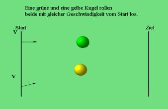
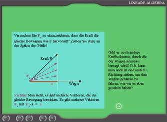
Velocity as a vector - application in physics: (Fig. 5): The learning environment will offer to the students the view onto applications of linear algebra. One of the basic examples in physics is the velocity, for which the direction is essential, not only the quantity. The animation can be repeated. |
|
|
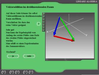
4 |
Multiple translations in the three-dimensional space - Three-dimensional topology (Fig. 6): Multiple parallel displacements in the three-dimensional space give an impression how the addition of vectors could be geometrically defined. The exercises should deepen this impression and pave the way to the concept of vector addition especially in three-dimensions. |
|
|
5 |
Addition of vectors in the 3-dimensional space - Three-dimensional topology (Fig. 7): These exercises give the students the chance to control there knowledge and skill in the vector addition. Again this task can be repeated as often as the students want. The new vectors will be randomly selected by the computer programme. |
|
In the same method the following exercises 6 to 8 will be offered:
|
6 |
Interactive addition of vectors - three-dimensional topology. |
|
7 |
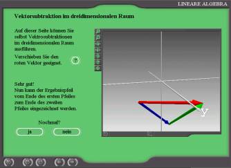
Subtraction of vectors in the 3-dimensional space - three-dimensional topology. |
|
8 |
Interactive subtraction of vectors - three-dimensional topology |
|
9 |
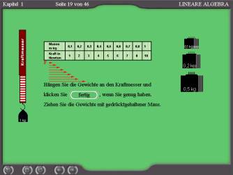
Multiplication of a vector by a scalar: Mass and force (Fig. 8): Measuring the weight (a vector) of masses one can multiply the masses and will get the multiple of the weight force. This pattern will illustrate the definition of the multiples of a vector (vector times scalar) which must will differ from the product of two vectors which will result in a scalar. |
|
|
10 |
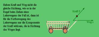
Scalar product of vectors (Fig. 9): The pattern is the well known trekking of a trolley, where the way has not the same direction as the force. The (physical) work is the model for the dot product of two vectors. |
|
|
|
The dot product is non reversible: There are many vectors which produce together with a given vector the same dot product. Fig. 10 shows how students can try out several vectors f (for the force) which have together with the vector s (for the way) the same work W representing the scalar product W = f . s . This is a very important insight. |
|
|
11 |
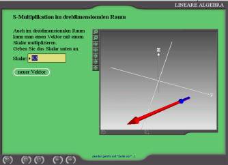
Multiplication of a vector by a scalar in the 3-dimensional space - Three-dimensional topology (Fig. 11): There are exercises for the multiplication of a vector in the three-dimensional space to give the students an impression of the geometrical multiplication of vectors. As before the picture can be rotated. All these tasks shall exemplify the vector space. |
|
|
12 |
Linear dependency and independency Solving a system of linear equations - concept of linear independency (Fig. 12): When students have to do this exercise the buttons shown in Fig. 12 are not all available, but only those for elementary operations to solve a system of linear equations. |
|

|
13 |
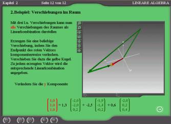
Linear combinations – concept: (Fig. 13). The task is to constitute a numerically given vector as a linear combination of three (numerically and geometrically) fixed vectors by multiplying the three vectors of the basis by the right coefficients. So students can learn the meaning of the linear combination and the basis. |
|
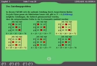
14 |
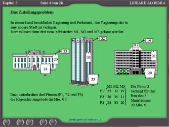
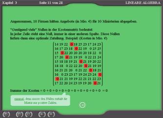
The problem of assignment: - Application of matrices (Fig. 14): The students will be familiarized with several applications of the linear algebra, especially of matrices. E. g. if three buildings should be built each by another of three building enterprises, how to choose the cheapest way? This is an application, where operations with matrices different from the elementary row (or column) operations are used. In the simple case of three buildings one can solve the problem “by hand” considering the various permutations, learning also the concept of permutations (see Fig. 15). For more extensive problems like choosing ten enterprises to build ten edifices one must use the matrix operations of the so called Hungarian method. The students learn how to use this method handling the matrices. Step by step they get the matrix, on which they can choose one of the possible permutations solving the given problem (Fig. 16). To learn various operations with matrices shall result in a better understanding of the concept of matrices and in a higher flexibility of thinking. |
|
|
|
||
|
|
|
15 |
Inversions - concept: Similarly there are tasks for getting the concept on inversions, which are required for the definition of the determinant function. |
|
16 |
Puzzle of Sam Loyd: An application of inversions will be shown by the puzzle of Sam Loyd. |
These are only some examples of topics, exercises and applications, which will be offered by the Computer aided learning environment for linear algebra.
The programme is developed by the “Arbeitsgruppe Computerlernumgebungen” at the mathematics department of the university in Koblenz (Germany)[9] in cooperation with the MuPAD research group at the mathematics department of the university of Paderborn (Germany)[10] and the publishing company Cornelsen in Berlin (Germany)[11].
The ongoing development of the learning environment can be watched at
http://euler.uni-koblenz.de/ag-clu/laufproj/mupadla .
Bridging the gap between
dynamic geometry and computer algebra:
The case of loci discovery
José L. Valcarce and Francisco Botana
Santiago, Pontevedra, Spain
2. Loci in dynamic geometry systems
3. A symbolic approach to loci equations and graphs
A basic problem in elementary geometry consists of finding the equation of a locus when giving some conditions, which define it. This problem has not been solved yet in the field of mathematics education from a technological point of view: There exists no friendly tool that allows a student to specify the conditions of a locus in a diagram and that returns the equation of the locus. Numerical approaches to this problem have been tackled in current dynamic geometry environments but they share essential incompleteness: an object must be constrained to move along a predefined path in order to get the trace of any other object. This paper describes a symbolic-dynamic approach to this problem: a computer algebra system solves it within a dynamic geometry environment.
1 Introduction
Dynamic geometry systems (DGS) were introduced in the secondary school in the 90s. These software packages enable users to build geometric figures on the screen. These figures retain their relationships and geometric properties when the user drags some geometric objects. In order to make the figures, every DGS provides tools for the construction of primitive objects (e.g., free points) and other derived objects (e.g., line through two points, parallel to a line through a point, circle with its centre in a point passing through another point, intersection points of two circles, etc.).
Dragging is the essential feature of these systems. Besides it, Cartesian coordinate systems, measures and equations of objects, macroconstructions, locus generation and a mechanism to record the history of the constructions are standard options in most DGS.
The Geometer’s Sketchpad (Jackiw, 1995), Cabri Geometry (Laborde …), Cinderella (Richter-Gebert and Kortenkamp, 1999) and Geometry Expert (Gao, Zhu and Chou, 1998) are well-known implementations of DGS. We will show the limitations of these packages when dealing with loci. We will describe Lugares, a new DGS that can communicate with two computer algebra system (CAS), Mathematica and CoCoa. In Lugares, numerical approaches to dynamic geometry can be complemented with the symbolic capabilities of CAS, letting a step forward to draw loci and find their equations.
2 Loci in dynamic geometry systems
There are two ways to draw loci in DGS
Trace of a point. A point A can be traced whereas another point B is dragged. The trace is the locus of A. This trace is not permanent (it vanishes when the dragging operation is finished).
Locus of a point A when another point B moves on an object. The trace operation can be automatically performed if B lies on an object. This locus is an almost dynamic object.
|
|
|
|
|
Fig. 1: The construction of two hyperbolas in a standard DGS |
||
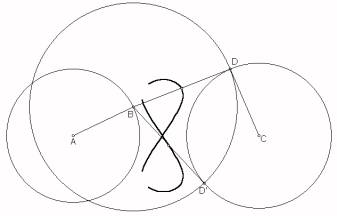
A hyperbola can be defined as the locus of points X such that the difference of distances to another points C and D is constant (distance(X,C)-distance(X,D)=k). Fig. 1 shows a segment AB, with length k, and a point C on the line AB. The difference between the lengths of AC and BC is k. In order to build the hyperbola, it is necessary to draw a circle with centre D and radius AC and another circle with centre E and radius BC. Let X1 and X2 be the intersection points of these circles. We have that distance(Xi,D) - distance(Xi,E)= AC - BC = k, and therefore Xi is on the hyperbola. The locus of Xi when C moves on line AB is the hyperbola. The incompleteness of the left hyperbola in Fig. 1 is due to the numerical approach, whereas the linear interpolation used to connect the trace points produces the anomalous hyperbola on the right.
DGSs
have four important limitations related to loci:
always need the construction of a point verifying the locus
conditions.
can only get the locus of a point that depends on another point
moving on a path (line or circle).
cannot get the locus of point such that other points depend on it.
cannot get the locus equation.
3 A symbolic approach to loci equations and graphs
Lugares is a DGS, developed in Visual Prolog, that uses a CAS for the loci discovery and graph. It can construct the hyperbola as follows:
Construct three points: A, B and X.
Define a reference system.
Introduce the condition distance(A,X)-distance(B,X)=2.
Tell the system, which the locus point, is.
Lugares deduces the polynomials associated to the relevant geometric conditions and gives this algebraic knowledge to a CAS (CoCoA or Mathematica). The CAS returns the locus equation, which can be plotted if wanted (Fig 3).
|
|
|
|
|
Fig. 2: Lugares can deal with metric conditions |
||
|
|
|
|
|
Fig. 3: The equation and the graph of the hyperbola |
||
4 A complete example
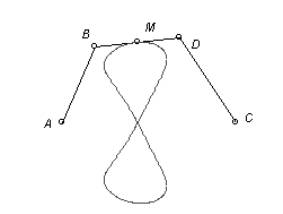
Let be a circle with centre O passing through A, and B another point on the circle. We search for the locus of a point X such that X is the midpoint of AB. This task can be easily done using a classical DGS since the locus of X depends on B, which lies on the circle. Nevertheless, the midpoint X of AB must be explicitly constructed. Using our approach, only the circle, the point B on it, and a free point X must be constructed (Fig. 4).
|
|
|
|
|
Fig. 4: The figure and the locus graph |
||
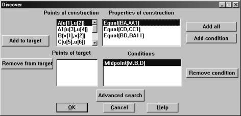
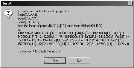
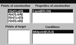
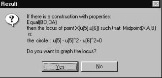
Adding the condition about X, (X is the midpoint of AB), the system knows that the construction can be described by a property (Equal(BO,OA)), the midpoint condition and a list of point coordinates (Fig. 5). Lugares generates the polynomials corresponding to the conditions and properties, and gives them to the CAS, where all the x variables are eliminated, returning the locus equation (Fig. 6).
|
|
|
|
Fig: 5: Part of Dialog window for Discover |
Fig. 6: The obtained result |
5 Implementation details
In this section we describe what is behind the interface. The basic idea is that in order to link algebra and geometry, we need polynomials. Therefore, the goal is to find a polynomial description of the given situation. The basic steps (Fig. 7) that Lugares performs to make these tasks are described using the example from above.
1. The construction is saved in a database of prolog facts, which contains all the geometric knowledge about the construction. We want to extract the geometric properties from it. Furthermore, we need to assign symbolic coordinates to each point in the construction. There are two models of points: free points and bounded points. Lugares assigns coordinates (u[#],u[#]) to free points and coordinates (x[#],x[#]) to bounded points. The algorithm that Lugares uses to get the properties and coordinates of points is simple:
Read object(Ref,Object,Label,_,_,_) of database
If Object=point then convert(point, geometric property)
The table shows the database of the example and the list of geometric properties that the convert predicate makes (column on the right).
object("1",point(161,179),"O",0,1,1) O(u[1],u[2])
object("2",point(261,179),"A",0,1,1) A(u[3],u[4])
object("3",reference1("1","2"),"",0,0,0)
object("4",line("1","2"),"X axis",0,0,0)
object("5",perpendicular("4","1"),"Y axis",0,0,0)
object("6",circle("1","2"),"c6",0,0,0)
object("7",point_on_object("6",0.8),"B",0,1,1) B(x[1],x[2]) ^ equal(BO,AO)
object("8",point(264,133),"X",0,0,1) X(u[5],u[6])
2. In the example there is only an additional condition: X is the MidPoint of segment AB, which is translated into midpoint(X,A,B).
3. The next step consists of getting the polynomials associated with the above geometric properties. This is an easy task because we have the coordinates of points that can be used to get the polynomials and we have a correspondence between geometric properties and polynomials. In our example, the translation between properties and polynomials is:
O(u[1],u[2])
A(u[3],u[4])
B(x[1],x[2])
X(u[5],u[6])
equal(BO,AO) ((0/100)-x[1])^2+((0/100)-x[2])^2-((100/100)-(0/100))^2-((0/100)-(0/100))^2))
midpoint(X,A,B). (u[5]-((100/100)+x[1])/2)
(u[6]-((0/100)+x[2])/2)
Note that the coordinates of O and A have been changed from (u[1],u[2]) to (0,0) and from (u[3],u[4]) to (1,0), respectively, since a reference system is defined.
4. All this information is passed to a CAS in a text file, whose content is:
Use R::=Q[x[1..2]u[1..6]];
C:=Elim(x,Ideal((u[5]-((100/100)+x[1])/2),
(u[6]-((0/100)+x[2])/2),
((0/100)-x[1])^2+((0/100)-x[2])^2-((100/100)-(0/100))^2-((0/100)-(0/100))^2));
MEMORY.LocusFirstCoord:=u[5];
MEMORY.LocusSecondCoord:=u[6];
MEMORY.Ref:=TRUE;
MaxMonomNo:=40;
<<'disclocus.coc';
CAS makes the elimination of every x[#] variable, the factorization and the classification of resulting polynomials (if possible).
5. When Lugares has the control again, it shows the result and the graph of locus.
|
|
|
|
|
|
Fig. 7: The basic steps in a loci discovery |
|
6 Conclusions
CAS and DGS have been developed independently, but when they work in cooperation they can improve the treatment of some geometric problems. This paper describes a computer program that fills the gap between both fields in the domain of loci discovery. It mixes techniques from both fields (computational commutative algebra and algebraic geometry, and dynamic geometry design) implying a step forward in the interactive exploration of geometric properties.
References
Gao, X.S., Zhang, J. Z.,Chou, S. C. (1998) Geometry Expert. Nine Chapters Publ. Taiwan.
Jackiw, N. (1997) The Geometer™s Sketchpad. Key Curriculum Press, Berkeley.
Kortenkamp, U. (1999) Foundations of dynamic geometry. Ph. D. Thesis, ETH, Zurich.
Laborde, J. M., Bellemain, F. (1998) Cabri Geometry II. Texas Instruments, Dallas.
Recio, T. (1998) Cálculo simbólico y geométrico. Síntesis, Madrid.
Richter-Gebert, J. & Kortenkamp, U. (1999) The Interactive Geometry Software Cinderella. Springer, Berlin.
Roanes Macías, E., Roanes Lozano, E. (1999) Búsqueda automática de lugares geométricos. Boletín de la Soc. “Puig Adam” de Prof. de Matemáticas-Congreso IMACS-ACA’99, 53, 67-77.
Valcarce, J. L., Botana, F. (2001) Lugares. Manual de Referencia. Techn. Rep., Univ.of Vigo, Pontevedra
[1] Axiom was developed by IBM with the colaboration of NAG, and previously named Scratchpad, was possibly the most powerful of all CAS, including what they called categories, i.e., the possibility to define the structure where calculations were going to take place, e.g. a non-commutative field. Normally all CAS work in polynomial rings or quotient fields over extensions of Ð. It has been surprisingly discontinued in 2001.
[2] A free version of MuPad for academic purposes exists.
[3] A Gröbner basis is a special kind of ideal basis that, once the order for variables and the kind of order to be used is fixed, allows to completely identify an ideal of a polynomial ring. Hence it is possible to solve difficult problems like if a surface is contained in a subspace of higher dimension. It also has many applications in different fields, like automatic theorem proving in Geometry, Logic, Robotics...
[4] Some DGSs (like Cabri Geometry II or Cinderella) include theorem-checking capabilities. Roughly speaking, Cabri's theorem-checker is based in altering the initial data: if it can find a counterexample then the result is false and it supposes that the result is true if it isn't able to find any counterexample. Therefore the truth of a result is not proved from the mathematical point of view. Cinderella's theorem-checker is more sophisticated but it doesn't prove the theorems (in the usual mathematical sense) either (Kortenkamp 1999).
[5] These assignings are slightly tricky, as they are done to variable-names themselves stored in variables.
[6] Observe that this is what happens in DGSs. Although initially not to intersect more than two objects seems to be a constraint or lost of time, forcing to intersect more than two objects would include the validity of a geometrical incidence theorem.
[7] This one doesn't exist in The Geometer's Sketchpad, but can be useful when directly working in Maple with the package.
[8] These relationships are necessary for instance when dealing with automatic theorem proving. The user knows where they are (in list LREL) and should add them wherever needed (e.g. to the set of hypotheses).
[9] Arbeitsgruppe Computerlernumgebungen am Mathematischen Institut der Universität in Koblenz, Rheinau 1, D-56075 Koblenz, Tel. +49-261-9119650, Fax +49-261-51976, email: w.fraunholz@uni-koblenz.de, http://euler.uni-koblenz.de/ag-clu
[10] MuPAD Distribution, AutoMath institute, University of Paderborn, Warburger Str. 100, D-33095 Paderborn, Tel. +49-5251-605533, Fax +49-5251-604209, email: distribution@mupad.de, http://www.mupad.de
[11] Cornelsen Verlag, Cornelsen Verlag, Mecklenburgische Str. 53, D-14197 Berlin, Telefon: (0 30) 897 85-0, http://www.cornelsen.de