Strand 4:
Changes in geometry and algebra
via Dynamic Geometry Systems
and Computer Algebra Systems
Hans-Georg Weigand
Würzburg, Germany
|
Plenary lecture: |
Fitting from function families with CAS and DGS |
|
A microworld for helping students to learn algebra |
|
|
Teaching and learning geometry: Dynamic and visual |
|
|
Dynamic notions for Dynamic Geometry |
|
|
Self-correction in algebraic algorithms with the use of educational software: An experimental work with 13-15 years old pupils |
|
|
A CAS-index applied to engineering mathematics papers |
|
|
Improving maths skills with CAS technology: A CAS project carried out in Scotland with 16-17 year olds using TI-92s |
|
|
Integrating MuPAD into the teaching of mathematics |
|
|
Absolute geometry: Discovering common truths |
|
|
Magic polyhedrons |
|
|
Cubics and quartics on computer |
|
|
Expression equivalence checking in Computer Algebra Systems |
1. Some changes in mathematics learning and teaching are necessary
2. The strand addressed especially the following questions
3. Conclusions of Strand 4 on changes in geometry and algebra
1 Some changes in mathematics learning and teaching are necessary
We are convinced that some changes in mathematics learning and teaching are necessary to give students more benefit from mathematics lessons for their future life. We are also convinced that new technologies will give us the opportunity to move in this direction. In strand 4 we discussed such changes while using the most important technological tools DGS and CAS (shortened in the following to: DaC). These consist of:
 changes in the contents of mathematics,
changes in curricula,
changes in teaching styles and the
method of teaching
changes in the way students learn
changes in concept formation
changes in assessment,
changes in working styles,
.....
2 The strand addressed especially the following questions
Contents of geometry and algebra
How can we reshape the contents of algebra and geometry programmes so that they have more immediate value to individuals? Can we identify explicit examples or ideas? What are the consequences for the curriculum? Which contents will take on increased importance, and which will decrease in importance?
Concept formation
With DaC, teachers can take new approaches to concept formation. Can these result in students gaining better understanding? What are the new difficulties? Will DaC give us an opportunity to make a better relationship between algebra and geometry?
Integration into the curriculum
For which students, and when, is it appropriate to introduce DaC? What are the benefits and the obstacles of an early use of DaC? What are the "by hand" skills, which should be retained?
Working styles
Will mathematical working styles change through the use of DaC?. Will this just be at the symbolic level, or will it affect graphical and numerical aspects. What is the relationship between working on the computer and working with paper and pencil?
Assessment
How will the means of assessment need to change when using DaC? Do we need new styles of test problems? Can traditional problems be modified for the "new" tests? Should DaC be allowed for every test?
If you see the literature, there are already a lot of proposals and suggestions for changes while using DaC: Reducing the complexity of hand-held calculations, giving more importance to experimental working, emphasising the modelling process and the interpretation of results - not "only" carrying out calculations, changes in assessment..... The goal of this workshop or strand was, to give an overview of the existing proposals for changes and to disseminate expected changes in algebra and geometry to teachers, math educators and administrators.
We were also interested in a close relationship of our strand to the discussion group for the 21st ICMI Study "The Future of the Teaching and Learning of Algebra"
(http://www.edfac.unimelb.edu.au/DSME/icmi-algebra/)
3 Conclusions of Strand 4 on changes in geometry and algebra
There was a wide spectrum in the topics of the lectures in strand 4 and if you ask for answers to the initial questions, you may be disappointed. But if you accept that it is impossible to answer questions concerning new technologies in general and when you are content with answers to special problems and questions, you may benefit from the discussions in strand 4. In the following there are a few conclusions and hypotheses for the future work with CAS and DGS, coming out of the presentations and discussions in strand 4.
We should put more emphasis on
CAS as a pedagogical tool in the classroom rather than a technical tool. We
have the possibility to explore algorithms, to visualise mathematical objects
and to illustrate procedures in new ways. The use of CAS and DGS allows us to
illustrate mathematical concepts and theorems, motivate applications and
re-introduce "tough" topics e.g. curvature.
The question of which kind of
CAS you use is of decreased importance. There are advantages of command-based programs
like MuPad or menu-based tools like Derive. It is not the way you use the tool
but the way you solve mathematical problems, which is important for the
development of mathematical thinking.
The visual and dynamic
abilities of interactive DGS can support “preformal proving”. This kind of
proof gains a special new quality by using DGS, which may be called
“visual-dynamic proofs”.
The use of visualisations and
multimedia animations in the classroom are wonderful new possibilities of
learning mathematics. But they also may cause additional problems for the
students because they have to develop first the understanding of these kinds of
presentations.
There should be – and there
will be – a real interactivity between DGS and CAS. More about spreadsheets
should be included in this joint-venture program. It should be easy to
transform data from one program to the other.
With Cinderella or
Java-Sketchpad you can work with DGS over the Internet. In the future it will
be possible to work with DGS, CAS and spreadsheets over the Internet.
It is still an open question
how to evaluate the level of difficulty of problems in assessment-tests, when
CAS are allowed. Some kind of “index” is needed to show the difference of the
level of a problem posed in a technology-free test or in a test where
technology is allowed.
Geometry should be studied more
from an experimental and inductive point of view. Especially DGS give the
chance to lay more evidence to this aspect. But students should also see
geometry as a formal system, a (local) axiomatic system, and a field of
exercise for proving,.
Programs like Cinderella allow
us to contrast different models of geometry, especially Euclidean and
Non-Euclidean Geometry.
Using computers enables us to
include objects into our lessons (at University) in an easy way, which are
described by algebraic equations of higher degree, for example cubics and
quartics.
CAS technology contributes to
the students’ learning and algebraic development but may also have a positive
effect on the development of maths skills. If students can make sense of the
mathematical procedures and get greater confidence in their work this will
result in a better understanding of maths skills.
In the future CAS and DGS will
have a tutoring component and may be extended to tutorial systems. But there is
still a lot to be done. The evaluation of the answers by students in the frame
of a tutoring system is a big challenge for the coming years.
Fitting from function families
with CAS and DGS
Jean Flower
Brighton, UK
2. Curvature and fitting circles at a point on the parabola
3. Best fit circles at arbitrary points on the parabola
4. Curvature on handheld technology
5. Fitting circles to any curve
6. Fitting a best fit parabola
The use of CAS and DGS allows us to illustrate existing work (e.g. eigenvalues), motivate applications of existing work (e.g. computer graphics and animation) and re-introduce "tough" topics (e.g. curvature). While CAS and DGS are used to investigate or resolve a problem, questions arise. These provide an opportunity to integrate side-topics into the main train of thought, and to include reflective thinking and analysis as part of an assessment process. In this article, I have chosen one mathematical area as a vehicle for illustrating the kinds of potential opened up by using DGS and CAS. The algebra involved would be challenging by hand, but could be brought back into the classroom (first or second year university degree level) with CAS as an algebraic support.
The chosen example concerns the "best fit" from a family of functions to a given curve at a given point. To start with, the family of functions will be the family of lines, and the chosen function will be a parabola. Later sections extend to other choices of curves and families. What’s interesting is not only how the problems and topics can be approached and what kind of mathematics evolves out of the study, but also what kinds of questions are raised in the process. These questions are highlighted in the article.
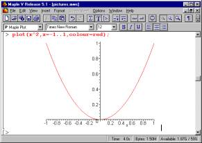
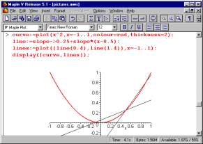
1 Tangents
The initial chosen task is to find a "best fit" line out of the family of all lines - find the best fit line at the point (1/2,1/4) on the parabola given by y= x2.
Question: What's a "family of curves"? Introduce the concept of a "parameter".
|
|
|
|||
|
Fig. 1: Plotting a parabola in Maple |
Question: How can you find the slope of the chord as the length of the chord shrinks to zero? Concept: limits, L'Hopital's rule.
Question: How was the graph of f (x) = x2 drawn in Sketchpad? (as a locus of points) How were the tangent lines drawn in Sketchpad? (only after following up the algebra)
A classroom activity asking "Which line fits best" can generate a dialogue "That one!" - "Which one?" and steers towards a common language for describing lines. A line can be specified by its slope, given a point of intersection with the curve. More generally, two points on the line could be given. Or some students may be more comfortable with the notation "y = mx + c".
Questions: What are the relative merits of the different representations of candidate lines? How can we convert from one representation to another? How come in one representation we have to give four numbers, in another we specify two, and in another, only one is required? Concept: degrees of freedom
A competitive edge can be introduced by getting students to provide information via their calculators to a central resource base (see reference for TI-interactive), which could display the on-going "votes" on screen. Repeating the competition for different choices of the underlying curve gives an atmosphere in which students can practise using the different representations of a line to cast their vote. Of course, every competition needs a clear winner as an outcome.
Questions:
How can we decide the democratic outcome of an election in which each vote is a line?
Does it make sense to average the m's and the c's?
If we arrived at an average line, how could we find which of the cast votes was closest?
Does the average give the best fit line? How can we decide what the best fit line is, anyway?
Concept: alternative distances or metrics in the set of lines giving different winners. The undemocratic nature of mathematical correctness.
2 Curvature and fitting circles at a point on the parabola
Calculus quickly helps us decide upon the best fit line from the family of lines. Extend the question to fit a circle to the parabola.
Question: How is the circle drawn in Sketchpad - as a function? using the toolbar?
Again, questions of representation arise. A circle can be specified by centre and radius, or by just a centre if a point on the circumference is given, or by a function.
Question: Which is the preferred representation of a circle? How many choices have to be made to specify a circle?
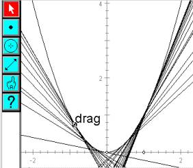
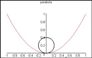
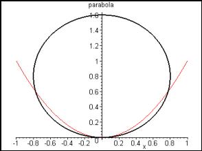
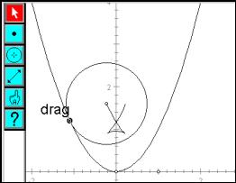
Using the circle toolbar button, a circle can be drawn with centre constrained on the vertical axis and circumference point at the origin. The size of the circle can be altered, ranging from circles, which are too small to those, which are too large. Some intermediate value must be "best".
|
|
|
|||
|
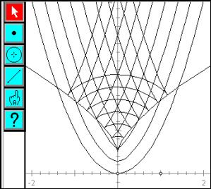
Fig. 7: Dynamic tangent circles in Sketchpad |
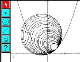
Fig. 8: The locus of centres with a small fixed radius |
Question: If students were to vote on the best fit circle, to get a feel for what should be roughly the "right" size, where could we expect the centres to lie? Is there a meaningful concept of an "average" circle? Or the vote that is "closest to average"?
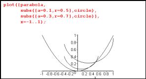
To vary the point of contact with the parabola, use centres of best fit circle candidates, which lie on the normal to the parabola. This leads to questions about the normal to a curve, and the relationship between the normal to a curve and the tangent. Figure 7 shows DGS being used to dynamically change the radius of a circle at a fixed point with the parabola.
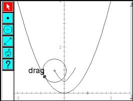
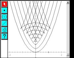
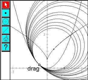
The same diagram, if carefully constructed, can be used to take an alternative slice through the family of circles? Figures 8 and 9 show DGS used to fix the radius and allow the common point to drag along the parabola. With a small, fixed, radius, the centre of the circle traces a u-shaped curve (not a parabola) inside the parabola. For a larger radius, locus gains two "kinks" (points at which the curve has no tangent) as the point on the parabola moves. These kinks must appear at some intermediate radius.
Question: What is the radius value, which is the smallest to produce a "kink" (a lack of smoothness in the locus)?
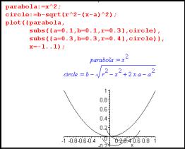
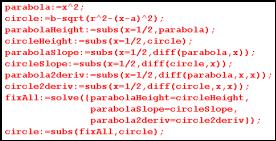
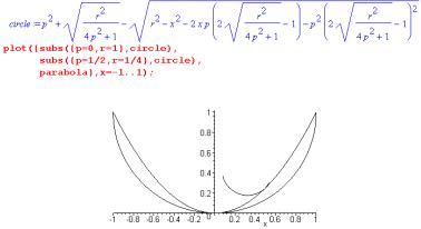
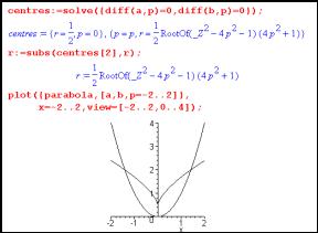
To investigate using Maple, set up expressions for the parabola and a circle. The circle expression is
![]()
where the centre is at (a,b) and the radius is r.
Question: Where did this algebra come from?
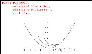
To plot instances of the circle, use the subs(…) function to substitute values into circle for a, b and r.
|
|
|
|||
|
Fig. 9: The locus of centres with a large fixed radius |
Fig. 10: Loci of centres for a range of radii |
|||
|
Question: The parabola and circle are, strictly speaking, expressions in Maple. To define the parabola as a function, we would write p:=x->x^2; What difference would this make? The circle expression, plotted against x, gives the lower semicircle, which will provide a better fit to the parabola than an upper semicircle. Question: Will it always be obvious whether to pursue the lower or upper semicircle for the best fit? |
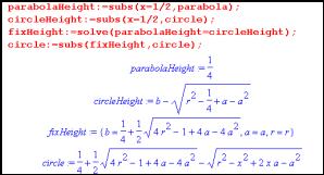
To find the best fit circle to the parabola point (1/2, 1/4), limit the family of circles to those, which pass through this point. Substitute the value x = 1/2 into the expressions for parabola and circle. Think of this as finding the "heights" of the graphs at x = 1/2. The solve facility is used to determine a condition on the parameters a, b, r. The parameter b is found in terms of the other parameters a and r. When this value for b is substituted into the circle expression, the family which used to depend upon r, a and b now only depends upon r and a. All circle graphs in the family pass through (1/2,1/4).
|
|
|
|||
|
Fig. 12: Maple algebra for matching the heights at (1/2,1/4) |
Question: Why was it the symbol b that was eliminated at this stage, rather than the alternatives r or a? Could we force Maple to follow an alternative choice?
Once the family of circles is restricted to those which pass through the point (1/2,1/4), a further restriction can be made which forces the slopes of the parabola and circle to agree. The slopes are found using the inbuilt diff function for differentiation. The parameter r becomes expressed in terms of a, and the circle family now has only one degree of freedom, through the parameter a.
|
|
|
|||
|
Fig. 14: Maple algebra for matching the slopes at (1/2,1/4) |

All members of the circle family are now tangent to the parabola at (1/2,1/4).
Question: Why did r become expressed in terms of a, instead of vice versa? Could we control the algebra to eliminate the parameters in a different order?
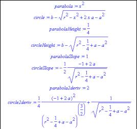
One final step allows us to fix the "best" circle as the one, which gets agreement for the second derivatives. The calculation for the second derivative is done using the diff( ) function, and yields a rather unpleasant-looking expression for the circle. However bad the algebra looks, the process has succeeded in producing a best fit circle to the given parabola point.
|
|
|
|||
|
Fig. 16: Maple algebra for matching the second derivative at (1/2,1/4) |
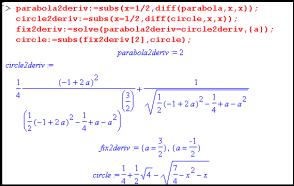

The family of circle has reduced to a single circle, with equation
![]()
Question: Why didn't Maple reduce the square root of 4 to 2, simplifying the expression?
|
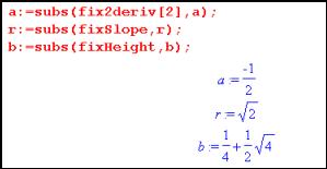
The conditions that have been found for the matching height, slope and second derivative can be used to find values for the centre co-ordinates and radius of the circle. Once we have a definitive result for the best fit, the votes in the competition can be reconsidered and the "best" vote found. |
|
|||
|
Fig. 18: Best fit circle parameters for (1/2,1/4) |
Question: Which of the circle votes were closest to this definitive best fit circle?
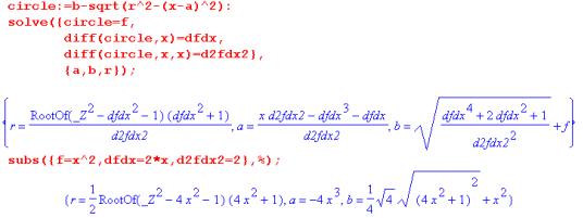
All of this work was done on Maple by copying the process we might take if we were to tackle the algebra ourselves. Maple is more powerful than we are in handling large expressions, and it's possible to challenge the program to take on more at once:
|
Fig. 19: Maple commands for finding the best fit circle quickly |
|
|
|
Fig. 20: The working for fitting at (1/2, 1/4) |
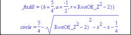
Build all the expressions needed for comparing heights, slopes and second derivatives. The solve() command can handle multiple simultaneous equations.
Question: What are the relative merits of working through a problem slowly in Maple compared to using fewer steps? Which is the preferred approach?
|
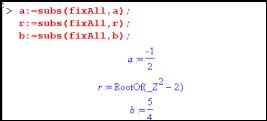
The values for a, b and r can be found, as before, using the three constraints for height, slope and second derivative, as shown in Fig. 21 |
|
|||
|
Fig. 21: Best fit circle parameters revisited |
The expression for the value of r in Figure 21 includes the phrase RootOf. RootOf(f (_Z)) means the (set of) possible value(s) of _Z as roots. For example, RootOf(_Z - 1) is the value +1, and RootOf(_Z 2 - 2) gives alternative values ±Ö2. The appearance of this forbidding notation shows that the choice between our two approaches can affect the appearance of the outcome.
Question: Why do the two approaches give different triples for a, b and r:
![]()
It's always worth trying the simplify() command when confronted by a complicated algebra expression. In this case, simplify(circle) does produce the earlier expression.
Question: Why doesn't Maple automatically simplify all its output?
3 Best fit circles at arbitrary points on the parabola
To study the best fit circle at an arbitrary point along the parabola, introduce variables p and q for the co-ordinates of a point on the parabola. The expressions for the parabola and circle are the same as before, and the process of finding matching height and slope is the same as before. The work we have to do is no more complex than for a single point (1/2,1/4), but the algebraic computation becomes trickier.
The derived expression for the circle is used to plot a tangent circle at any point on the parabola:
|
|
|
|
|
|
|
Fig. 22 |

The centre of any tangent circle is found in terms of the parameters p (for the tangent point) and r (for the circle radius)
|
|
|
|||
|
Fig.23a: Centre co-ordinates for an arbitrary tangent circle |
Fig.23b: The locus of centre as the radius changes |
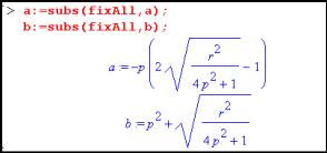

Fig. 23 shows a and b plotted to give a parametric curve as r changes - the locus of centres of circles at a fixed point for fixed p (value = 1/2) with varying radius r. This locus is a straight line - a segment along the normal to the curve.
Fig. 24 shows a more interesting curve, created by varying p and leaving r fixed (value 3/2). This is the locus of centres as a circle of fixed radius moves along the parabola.
|
|
|
|||
|
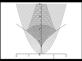
Fig. 25: Centre loci for a range of radii |
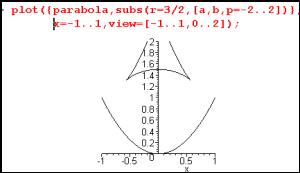
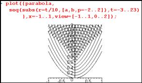
Fig. 25 shows the family of centre loci for fixed radius; fix the radius to be a family of values from 3/10 to 23/10. It recreates the DGS loci shown in Fig. 10. Where are these "kink" points? (Points at which the curve is non-differentiable) Given the parametric points (a, b), with parameter p imagine a point travelling along the locus as p changes. The kink shows that the point stops moving to the right, turns round, and starts moving to the left. It also stops moving upwards, turns round, and starts moving downwards. The expressions for a and b must have stationary points.
|
|
|
|||
|
Fig.26a: The locus of kinks |
Fig.26b |
More Maple work can be done to match the second derivatives and derive best fit circle centres. Plotting the best fit circle centres matches the "locus of kinks". The algebra can be seen to be the same, as illustrated here in Sketchpad.
Using the second derivative as the definition of "best fit" is proved to match the more intuitive definition of "critical radius" - a radius that produces a kink in the locus of centres for fixed radius.
4 Curvature on handheld technology
It would be easy to imagine that the Maple program, running on a powerful PC, is capable of this kind of algebra where handheld technology could struggle. As shown below, the TI89 has no problem in reproducing this work. The following screen dumps are taken from the inbuilt text editor to tell the story interspersed with command lines. The resulting algebra is in some cases too large to fit on the screen.
|
1. |
2. |
3. |
|
|
|
|
|
|
|
|
|
|
|
|
Questions: Why solve for b? Is there a better way to refer to the solution for b, other than copying and pasting from the home screen? |
Question: If b has been given a value, is c(…) still a function with four parameters? |
||
|
4. |
5. |
6. |
|
|
|
|
|
|
|
|
|
|
|
|
Question: Why are there two results for a? What if we had chosen to solve for the parameters a, b and r in a different order? |
Question: Which solution for a is the right one to use for the next step? Use a parametric plot to fix values of r (values fixed as 0.3, 0.4, .., 1.3) |
Plot the centre co-ordinates (a,b) as p changes. Question: why is it necessary to use xtemp and ytemp here? |
|
|
7. |
8. |
9. |
|
|
|
|
|
|
|
|
|
|
|
|
Question: Why not type solve(d(d(f(x),x),x)=d(d(..? instead of evaluating the derivatives and copying them into the solve expression? |
Question: Why did the solve ( ) command give multiple results? Which one was chosen and why? |
Question: Would the plots appear faster if these expressions were evaluated on the home screen and the output pasted into the Y= screen? |
|
|
10. |
|
11. |
|
|
|
Question: Why do these circles have gaps at the sides? |
|
|
|
|
Would there be any way of plotting the circles to avoid this problem? |
|
|
5 Fitting circles to any curve
The Maple algebra can be generalised to fit circles to any curve, giving curvature formulae for the best fit centre and radius.
|
|
|
|
This result for the general best fit radius and centre can be written as
|
|
|
|
This could be applied, for a different example, to fit a circle to a sine wave:
|
|
Question: How can we create an image of the sine wave? How can the derivatives of the sine curve be found in Sketchpad, for plugging into the curvature expressions? Fig. 28 shows the locus of centres of the best fit circles. |
|
Fig.28: Best fit circles to a sine wave |
|
|
|
|
|
Fig. 29: Best fit circle and centre locus |
Fig.30: Loci of centres for a fixed, small, radius |
|
Fig. 31: Loci of centres for a fixed, large radius |
Fig.32: Loci of centres for a range of fixed radii |
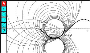
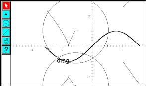
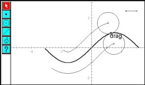
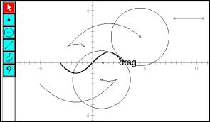
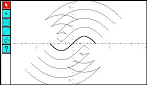
Figure 30 to 32 show the loci of centres of circles with a fixed radius. Again, we see the introduction of non-differentiable points (kinks) for larger radii.
Question: Will such kinks always occur for any choice of curve?
|
|
|
|
Fig. 33: Algebra for curvature of sine waves |
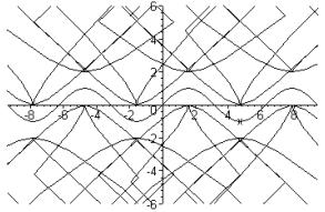
Fig. 33 shows the kind of algebra that Maple produces in the analysis of fitting circles to a sine wave. The algebra is forbidding and gives the impression that we would never be able to recreate the result by hand. The commands typed in, however, are no more complex than used when fitting circles to parabolae.
Question: Could we recreate such forbidding algebra by hand? Would we want to? What would that teach us?
6 Fitting a best fit parabola
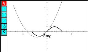
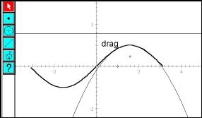
The construction of the parabola in Figure 35 was done by plotting the function
![]()
The responsiveness of the image is limited by the amount of calculation to be done at each stage, as the point is dragged along the sine wave. The construction of the circle as a locus of equidistant points gave a smoother outcome in the curvature work. To improve the responsiveness of the best fit parabola, it could be possible to reconstruct the parabola as a locus of equidistant points between a focus and directrix. This drives some more algebra. How can we convert from the quadratic polynomial representation of the parabola to a focus and directrix? The focus is a point somewhere in the plane, and the directrix is a horizontal line, specified by its height.
The quadratic x2 has focus at (0, ¼)) and directrix at height –¼ . In order to generalise to an arbitrary quadratic, we need to understand the roles of the coefficients a, b and c.
|
|
|
|||
|
The approach used to find a best fit circle can easily be applied to find best fit parabolae. The images can be constructed statically or dynamically. But one issue arises which leads back to paper and pencil constructions of parabolae. |
|
|||
|
|
Fig. 35 a-c |
|
Completing the square gives |
|
|
|
The parabola has been shifted by |
|
and scaled vertically by a. |
|
The focus becomes |
|
and the directrix at height – ¼ a. |

Question: How does the notion of shifting and stretching change the algebra for focus and directrix?
|
|
|
|||
|
Fig. 36: Parabola plotted from directrix and focus |
Fig. 37: Focus locus for best fit parabolae |
7 Conclusions
This work was about fitting from function families. It could have been about many other topics - the issue under consideration is to think about the experience of doing mathematics aided by CAS and DGS. The questions raised make links from this specific investigation about to wider issues from both geometry and algebra:
alternative algebraic representations; metrics on spaces; smoothness; loci, paper and pencil constructions; degrees of freedom; Taylor series, limits; strategy in algebra work; tangents and normals; families and parameters; Cartesian and parametric forms for graphs; multiple solution sets; correctness; effects of scaling and stretching on algebra; where algebra comes from;…
The most commonly phrased questions are of the form:
Why did the technology do this? / How to make the technology do
that…?
How to decide between…
How to find …
Does it make sense to…
Consideration of these questions helps to create a coherent understanding of the subject. Even the questions, which appear to relate directly to understanding the technology, instead of the maths, often disguise mathematical ideas about dependency between objects, or using different expressions for the same thing.
We could set ourselves the task of following behind the CAS tools, trying to match their algebraic techniques and repertoire by hand. An alternative approach opens up higher conceptual questions about how topics link together, dependency between mathematical objects, steps in mathematical investigation and proof. It could be argued that in this study of curvature, algebra has been acting as the tool for investigation rather than comprising the focus of the task in hand. What drives the work forward is curiosity about the algebraic expressions and the images produced.
The questions that have been emphasised in this work could act as part of an assessment strategy. Students could be challenged to come up with questions. A fun way to present the rich structure of ideas could begin with a description, as given here, on a web page. Students could add their questions into the text as hyperlinks to their own pages with discussions of the different points raised. Both Sketchpad and Cabri can produce Java scripts, and so dynamic images can form an integral part of work on a web page.
8 Resources
|
Technical: |
|
|
TI89 syntax: |
http://education.ti.com/product/tech/89/guide/89guideus.html |
|
TI interactive: |
http://education.ti.com/product/software/tii/features/features.html |
|
Maple CAS: |
|
|
Geometer's Sketchpad: |
|
|
Java Sketchpad: |
|
|
A paper including work on fitting tangents: |
|
|
Jean-Baptiste Lagrange: "A didactic approach of the use of CAS to learn mathematics" CAME '99 at |
|
|
|
|
Acknowledgement. Thanks to Adrian Oldknow and Warwick Evans for inspiring me to take CAS on board, years ago. Thanks to TI for the calculator, and to Paul Harris for his help with Maple syntax.
A microworld for helping students
to learn algebra
Denis Bouhineau, Jean-François Nicaud, Xavier Pavard, Emmanuel Sander
Nantes, Paris, France
2. What can be a microworld for algebra
3. Main actions of the editor of an algebraic microworld
5. The Aplusix microworld for algebra
6. Domain of validity and discussion
This paper describes the design principles of a microworld devoted to the manipulation of algebraic expressions. This microworld contains an advanced editor with classical actions and direct manipulation. Most of the actions are available in two or three modes; the three action modes are: a text mode that manipulates characters, a structure mode that takes care of the algebraic structure of the expressions, and an equivalence mode that takes into account the equivalence between the expressions. The microworld also allows to represent reasoning trees. The equivalence of the expressions built by the student is evaluated and the student is informed of the result. The paper also describes the current state of the implementation of the microworld. A first prototype has been realised at the beginning of February 2001.
1 Introduction
Mathematical microworlds have been developed since the late sixties. The first one was Logo (Papert 1980) devoted to recursive programming and geometry. The concepts of mathematical microworld have been established in the mid and late eighties (Thompson 1987, Laborde 1989, Balacheff and Sutherland 1994), and the main features have been exhibited: objects, relationships, operators and direct manipulation. Several microworlds have been realised in geometry and algebra. Some of them are distributed has commercial products and have (or have had) a real success, like Logo and Cabri Geometry (Laborde 1989). The last one has been implemented on pocket calculators and distributed as computer software by Texas Instruments. Microworlds for geometry provide a real contribution to the learning of the domain and have introduced a new concept of geometry called dynamic geometry.
In this paper, we consider microworlds for formal algebra. Algebraland (Foss 1987) and the McArthur’s system (McArthur e.a. 1987) can be seen as the first ones. Others software for algebra, like those devoted to the modelling of word problems (Koedinger e.a. 1997), are not concerned here. In our previous works, we realised what we consider as second order microworlds for algebra. Ours systems were advanced prototypes (Nicaud e.a. 1990, 1994). We conducted a lot of experiments and analysed students’ behaviour and learning using these systems (Nguyen-Xuan e.a. 1993, 1999). We are now designing and realising what we consider as a first order microworld for algebra. This system aims at becoming a commercial product. In the future, we will combine the features of first and second order microworlds.
The fundamental question is: What can be a microworld for algebra? In this paper, we define first and second order microworlds. Then we detail first order microworlds and describe the mains specifications of the system we develop and the current state of its realisation.
2 What can be a microworld for algebra
According to Laborde (1989) a microworld is a world of objects and relationships. There is a set of operators able to operate on the objects to create new ones with new relationships. Direct manipulation has an important place in microworlds. Balacheff and Sutherland (1994) emphasise on an epistemological domain of validity providing the relationship between the representations and what they intend to represent. Thompson (1987) tells that mathematical microworlds must facilitate the process of constructing objects and relationships and focus on the construction of meaning. They must use a model not embedded in the curriculum, they must not provide instruction.
In formal algebra, as said above, the concrete objects are expressions. The basic relationship between the objects is the structural relationship over the expressions: 12 is the first argument of the second argument of
![]()
The second relationship is the equivalence relationship. There are two main sorts of operators.
The first sort operators allow building any well-formed expression: they are the operators of algebraic expression editors. We term first order the algebraic microworlds that focus on these operators. First order algebraic microworlds are included in many word processing systems. They are called equation editor. We will show below that most of them have a poor relationship with the semantic objects of algebra. The McArthur’s system (McArthur e.a. 1987) has feature of a first order algebraic microworlds.
The second sort operators are the transformation rules that allow building new steps in a reasoning process. We term second order the algebraic microworlds that focus on transformation rules. Several second order algebraic microworlds have been realised in the past (Bundy and Welham 1981, Foss 1987, Thompson 1989, Oliver and Zukerman 1990, Beeson 1996). The previous systems we developed in our team were of that class. Students solved problems by applying transformation rules to selected sub-expressions. They were not allowed to build a step another way. The community did not really consider these systems as microworlds, may be because they teach (something refused by Thompson), may be because they do not have the first sort operators, may be because people who realised these systems emphasised more on the tutoring aspects.
In the rest of the paper, we focus on first order algebraic microworlds we just call algebraic microworlds. In section 3., we consider the classical features of an editor for an algebraic microworld. In section 4., we tackle the issue of direct manipulation.
3 Main actions of the editor of an algebraic microworld
Objects and the structural relationship
A microworld must allow the user to create objects. In the case of algebra, this means to have an editor for algebraic expressions. The visual fidelity imposes the usual 2D representation for the interface of the editor. This representation contains text parts that can be seen as successions of characters
|
like 2x+1 |
and bloc parts well delimited like |
|
and |
|
The conceptual fidelity imposes to take the structural relationship into account. So, we propose to give to students well-formed expressions, as much as possible. For that purpose, expressions with missing arguments are completed with something, for example “?” (e.g., typing + at the end of 2x provide 2x + ?) and expressions that cannot be completed are highlighted (as spelling errors in MS-Word).
The main actions of an editor are: input, delete, select something, apply an operator to something, copy something, delete something, cut something, paste something. Let us consider these actions through the structural relationship. This implies that the above something is a sub-expression. We call the structure mode, a mode where well-formed sub-expressions are preserved during the actions and text mode, a mode where well-formed sub-expressions are not preserved. Note that the two modes are useful, the former to avoid destroying what is already built, the later to let the user be able to do everything.
Proposals for the implementation of the actions
Input from the keyboard (or input by clicking a button), when the expression has an insertion point: in order to keep a well formed expression, the input of a text operator adds “?” when necessary; in the structure mode, the input of a bloc operator adds “?” for each argument; in the text mode, the input of a bloc operator uses the environment for the arguments (e.g., typing / after x in xy provides x/y).
Select a sub-expression: the structural relationship suggests selecting only well formed sub-expressions. Note that 2x + 4 in 2x + y + 4 and –mp in 1 – 2mxp are well-formed sub-expressions. The natural idea for the selection is to consider the smallest sub-expression that includes the dragged area. Such actions were implemented in our previous prototypes and were appreciated by the students and the teachers.
Reasoning and the equivalence relationship
An important activity in formal algebra consists of solving problems by successive transformations of expressions, with conservation of the equivalence. After the edition of expressions we have to consider the representation of the reasoning processes for an algebraic microworld. A reasoning process contains not only successive transformations of expressions, with conservation of the equivalence, but also backtracks and sub-problems. A backtrack is sometimes realised when solving a problem. It consists of going back to a former step to try another way to solve the problem (so the steps have the form of a tree). A sub-problem is sometimes extracted and solved to help to solve a problem. Given a problem <T e>, T being the type and e the expression, the most frequent situation for a sub-problem consists of having a problem <T1 e1>, where e1 is a sub-expression of e, such that the solved form of the sub-problem may benefit to the original problem. For example, <solve A=0>, when A is a polynomial having a degree higher than 1, benefits from the resolution of the sub-problem <factor A>.
We consider that an algebraic microworld must represent reasoning processes, the equivalence between expressions, backtracks and sub-problems.
Propositions for the implementation of reasoning processes
In our previous prototypes, we implemented all the above features. The link between equivalent steps was an arrow and corresponds to a tutored action. We think now that it would be more accurate for an algebraic microworld to use a double arrow meaning “these expressions are equivalent”. Backtrack was implemented by the possibility to have several successors to any step. We think good to keep that. Sub-problems were linked to problems with a special arrow. We think now that it would be better to solve sub-problems on other places of the sheet or on other sheets. As for the expressions, the system must highlight the expressions that are not equivalent.
4 Direct manipulation
In a microworld, direct manipulation allows to displace objects taking into account the relationships. Expressions, sub-expressions and operators can be manipulated through the structural and equivalent relationships or without taking care of these relationships.
Drag & drop a sub-expression
A selected sub-expression s can be dragged & dropped inside an expression e as a word in a word processing system. Such action changes the expression. Let us call u the expression obtained. In the structure mode, the constraints we consider comes from the structural relationship, they are: (1) u is a well formed expression, (2) s is a sub-expression of u, (3) sub-expressions of e that does not include s are left unchanged. Note that these constraints introduce sometimes parentheses around s. In the text mode, the only constraint is the first one and parentheses are never added. When s is a sub-expression of u, s is still selected and a new drag & drop may be performed. In the text mode, when s is not a sub-expression of u, there is no selection in u at the end of the action, see an example in section 5, Fig. 3. The aim of drag & drop in these two modes is to allow the user to build the expression (s)he wants to.
The aim of drag & drop in the equivalent mode is very different; it is to maintain the equivalence. So we add constraint (4) u must be equivalent to e. With constraints (1) to (4), the only general move that can be done consists of displacing an argument of a commutative operator. To get a more powerful equivalent drag & drop, we withdraw constraint (3) so that sub-expressions of e that does not include s may be changed.
Let us take as an example the expression (y-1)(x+x2), select the first occurrence of x and drag it between the two parentheses. We may expect to get (y-1)x(1+x) which is a factorisation. An explanation for factoring in such context may be that the moved expression is an argument of a sum, which is an argument of a product, the action being performed as “get x as a common factor of the sum and insert it as a factor of the product”. Note that it is necessary to withdraw constraint (3) for that, because x2 has been changed in x.
5 The Aplusix microworld for algebra
Our team planed to realised a first order algebraic microworld in September 2001. The Aplusix microworld will include two main activities: first to allow the student to build expressions, second to allow the student to solve a problem on an algebraic expression. A first prototype has been realised at the beginning of February 2001 and a first experiment is planed for mid 2001. The recording of the interactions is already implemented. Every elementary action is recorded in order to analyse the students’ behaviour in the laboratory by hand or by programs. The first experiments will be conducted with 15 years old students in the mid 2001 in order to evaluate the two activities.
The development is realised with Borland Delphi for windows. It current state is described here.
The 2D display of expressions is implemented with the following operators: + - ´ / ^ Ö = ¹ < > £ ³ and or not. The selection, including the selection of several arguments of a commutative operator) is implemented (see Fig. 1). Insert, delete, copy, cut, past are implemented in the text and structure modes.
The display of the reasoning tree is implemented (Fig. 3). The evaluation of the equivalence of two expressions A and B is realised when A and B are polynomials of one variable and when A and B equations with one unknown and a degree less than 4.
The direct manipulation is implemented in the text and structure modes (Fig. 2). The equivalent drag & drop is implemented only for moving an argument in a commutative operator. A complex equivalent drag & drop is not necessary for our first experiments with 15 years old students and needs a deeper reflection; our goal is not to implement a pretty mechanism but a mechanism having an epistemological value.
![]()
Fig. 1: Display of an expression in the usual 2D representation with selection
|
|
|
|
|
Fig. 2: A drag & drop. The selected expression
(on the left) is dropped between 2 and y |
||
|
|
|
|
|
Fig. 3: A reasoning tree with non equivalent expressions |
||
Later realisations in the framework of our first order algebraic microworld will include: (1) the representation of new operators, a column operator to represent systems of equations in the usual form, å, ò, etc., (2) a powerful equivalent drag & drop (3) the manipulation of fraction bars and radicals, (4) the representation and display of sub-problems, (5) the extension of the evaluation of the equivalence (we will use results of applied mathematics and constraint programming), and (6) a redisplay function. Of course, we will also add features or realise modifications suggested by the experiments.
We plane to combine next this microworld with our previous works, adding transformations rules, knowledge to solve problems, to evaluate students’ resolutions, to explain, to provide hint.
6 Domain of validity and discussion
To conclude, we would like to discuss the domain of validity as emphasised by Balacheff & Sutherland (1994) who defined fours dimensions in mathematics for the epistemological domain of validity:
The first dimension is the set of problems, which the microworld allows to be proposed. For the building expression activity of the Aplusix microworld, it is any well-formed expression using the operators and the constants included in the system and respecting the types. For the reasoning activity, the set of problems is constituted by any problem concerning an algebraic expression that belongs to the class of expressions the system is able to compare for the equivalence relationship. It is currently the polynomials of one variable with any sort of form and any sort of coefficients and equations with one unknown having a degree less than 4. Other classes of expressions will be added later. Note that this is independent of the problem type (factor, expand, solve, etc.). The problem type must just be an algebraic problem type, i.e., must be such that a problem is invariant when the expression is replaced by an equivalent expression.
The second dimension is the nature of the tools and the objects provided by its formal structure. The objects of the Aplusix microworld are algebraic expressions as they are defined in the rewrite rule theory (Dershowitz and Jouannaud 1989), which is the most achieved theory on expressions. The nature of the tool is to allow to build expressions and to allow comparing expressions according to the equivalence relationship.
The third dimension is the nature of the phenomenology over its formal structure. The phenomenology at the interface of the Aplusix microworld has a maximum of fidelity concerning the representation of expressions. It is our permanent first principle for the interface: implement the usual 2D representation. Concerning the edition features, as exposed in this paper, we defined them using fundamental concepts of the domain (the structure and equivalence relationships). The display of the equivalence is a natural phenomenon as the equivalence is a fundamental feature of any algebraic reasoning.
The fourth dimension is the sort of control the microworld makes available to users and the feedback provided. For the building expression activity, the student may execute any editing action. The major difference with other editors is that ill-formed expressions are highlighted. Most of the time, actions that lead to incorrect expressions are completed in order to get a well-formed expression (instead of refusing the action). This is a form of feedback. When the student disagrees with the interpretation of the system, (s)he can undo the action. For the reasoning activity, the student may produce a new step at any time and has the indication of the equivalence as fundamental feedback. This category of feedback, already realised by McArthur (McArthur e.a. 1987) in an elementary context, has not been deeply experimented. We are impatient to observe how it can benefit to the students’ learning.
Balacheff & Sutherland (1994) also evoked a didactic domain of validity for microworlds. On that issue, we will just indicate two points. First, the Aplusix microworld is fundamentally an algebraic world, not a pre-algebraic one. For example, there is no subtraction in it. The minus sign is a unary symbol ( a-b is the sum of a and the opposite of b). So students who are not ready to be plunge into a strict algebraic context will probably not benefit from the use of the system. Second, the system can be parameterised by the user or the teacher. A text file contains the description of the operators. It is possible to activate or deactivate an operator; it is possible to change some feature of an operator. For example, one can allow or not variables in a denominator or in a square root. These parameters allow to custom the environment to a particular level.
We have designed an algebraic microworld an epistemological way, and we are ending the first prototype. We hope that most of our choices will be good, but we are not sure. The answer will come from the users and we will analyse carefully the discrepancies between the behaviour of the system and the user expectations, in order to correct minor problems and to learn from the major ones and correct them too. Major problems, and the lesson they provide, will be published.
References
Adobe FrameMaker V5.0 http://www.adobe.com/products/framemaker/main.html
Balacheff, N., Sutherland, R. (1994) Epistemological domain of validity of microworlds, the case of Logo and Cabri-géomètre. Lewis, R., Mendelsohn, P. (eds.) Proc. of the IFIP.
Beeson, M. (1996) Design Principles of Mathpert Software to support education in algebra and calculus. Kajler, N. (ed.) Human Interfaces to Symbolic Computation. Springer.
Bundy, A. and Welham, B. (1981) Using Meta-level Inference for Selective Application of Multiple Rewriting Rule Sets in Algebraic Manipulation. Artificial Intelligence vol 16, no 2.
Dershowitz, N., Jouannaud, J.P. (1989) Rewrite Systems. Handbook of Theoretical Computer Science, Vol B, Chap 15. North-Holland.
Foss, C.L. (1987) Learning from errors in algebraland. IRL report No IRL87-0003.
Graphing Calculator V1.2 http://www.pacifict.com/
Koedinger, K.R., Anderson, J.R. (1997) Intelligent Tutoring Goes To School in the Big City. International Journal of Artificial Intelligence in Education 8, 30-43. 1997.
Laborde, J.M. (1989) Designing Intelligent Tutorial Systems: the case of geometry and Cabri-géomètre. IFIP Working Conf. Educ. Software at the Sec. Educ. Level, Reykjavik, 1989.
McArthur, D. Stasz, C., and Hotta, J.Y. (1987) Learning problem-solving skills in algebra. Journal of education technology systems 15, 303-324.
Microsoft Equation V3.0 http://www.mathtype.com/msee
Nguyen-Xuan, A., Nicaud, J.F., Gélis, J.M., Joly, F. (1993) An Experiment in Learning Algebra with an Intelligent Learning Environment. Actes de PEG'93, Edinbourgh.
Nguyen-Xuan, A., Bastide, A., Nicaud J.F. (1999) Learning to match algebraic rules by solving problems and by studying examples with an intelligent learning environment. Proc. AIED’99.
Nicaud, J.F. Aubertin, C., Nguyen-Xuan, A., Saïdi, M., and Wach, P. (1990) APLUSIX: a learning environment for student acquisition of strategic knowledge in algebra. Actes de PRICAI’90. Nagoya.
Nicaud, J.F. e.a. (1994) The APLUSIX project: a computer-aided teaching of algebra. Methodology, theoretical foundations, realisations and experiments. CALISCE 1994.
Oliver J. and Zukerman I. (1990) Dissolve: An Algebra Expert for an Intelligent Tutoring System. Proceeding of ARCE. Tokyo.
Papert, S. (1980) Mindstorms. Children Computers, and Powerful Ideas. Harvester, Sussex.
StarOffice V5.1 http://www.sun.com/staroffice
Thompson, P. W. (1987) Mathematical Microworlds and Intelligent Computer Assisted Instruction. Artificial Intelligence and Instruction, Addison Wesley, Reading MA.
Thompson, P. W. (1989) Artificial Intelligence, Advanced Technology, and Learning and Teaching Algebra. Wagner, S. and Kieran, C. (1989) Research issues in the learning and Teaching of Algebra. Lawrence Erlbaum.
Full paper: http://www.sciences.univ-nantes.fr/info/recherche/ia/projets/aplusix/
|
|
|
|
1 Geometric tools and constructions
For thousands of years compass and straightedge (ruler without scale) were the traditional tools of Euclidean geometry. Geometrical objects were points, straight lines, circles, triangles/quadrilaterals and so on. Rulers with scale and protractor became standard tools hundreds of years ago and consequently the length of segments, the size of angles, areas, and coordinates of points have become geometrical objects. Traditionally (in Germany) a student first does the construction and then writes down a description of how they carried out the construction.
In the 80's a type of geometry software became available with which one could do exactly the same constructions as with compasses, ruler and protractor. Constructions were made in an editor by typing special commands. The aim was to construct special triangles with given properties. It was static software. Because there was no real advantage other than being able to have an accurately printed sketch, this geometry software was not successful in the classroom.
In the late 80's and the 90's dynamic geometry software (DGS) was developed (Cabri Géomètre, Geometer's Sketchpad) and began to be used in teaching geometry. Constructions were now done by mouse-clicks on a graphic surface, with the DGS automatically producing a sequence of construction-commands. The aim was now not the construction of special triangles, but the investigation of invariances, functional dependencies and loci.
2 Special qualities of DGS
With DGS one can produce all the constructions which were possible with compasses, straightedge, ruler and protractor. Furthermore new abilities are added by dragmode and loci. This requires a deeper understanding of the construction and the sketch. Two sketches which look identical on the screen can show a completely different behaviour when they are being dragged. 'Drag-stability' becomes an important criterion for the correctness of a construction, something which was not applicable to paper & pencil constructions.
The distinction between drawing(= ‘Zeichnung’) and figure (= ‘Figur’) has been formulated for DGS by Parzyzs and Strässer, but it is was completely clearly formulated by Strunz (1968), who pointed out “die Idealität der geometrischen Figur, die eben doch etwas anderes ist als eine bloß retouchierte visuell wahrnehmbare Zeichnung” (= the ideality of the geometric figure, which is other things than a simply touched up visual perceptible drawing). In the dragmode, as can be seen on the screen instantly, the drawing can be changed. Hence the drawings represents the basic geometric relationships; it can be seen as the class of all drawings with the same properties and the same relationships. It will not be changed by dragging. The aim of constructing is not to construct a special sketch, but to construct a figure and to investigate its properties, to examine what changes and what remains invariant. The figure is represented in the DGS by a sequence of construction-commands or a construction-program. In the dragmode this construction-program will start again and again with varied inputs.
Furthermore a deeper understanding of degrees of freedom (= 'Freiheitsgrad') and of geometrical dependencies is necessary. We have several kinds of points: a free base point has two degrees of freedom and can be moved at will in the plane / on the screen. A point on an object has one degree of freedom and can be moved on a straight line or on a circle and in some DGS can also be moved on a conic or other figures. An intersection point has no degree of freedom; it can be moved only indirectly by dragging the base objects. Similarly several kinds of line-segments and circles exist.
In the dragmode it is possible to measure length, angles or areas dynamically and it is possible to calculate with these dynamic measures and to make further dynamic constructions using these results. This offers new opportunities for finding and/ or testing conjectures!
Examples of special DGS-qualities:
(To return please use the Back-Button)

3 Formal proofs
For more than 2000 years the teaching of geometry has been influenced by formal proving following Euclid. A proof is made line by line, drawing logical conclusions from conditions and known theorems, without consideration of concreteness. This is the way scientific results are normally presented, but it is well known that it is not the way students learn geometry. Asked the classical question "Wie lernt jemand das Beweisen?" (= How to learn proving?) most people give the classical answer "Indem man ihn Beweise lehrt" (= by teachìng proofs) and "und sie ist, wie man weiss, untauglich." (= but it is - as we know – of no use.) (Freudenthal 1979).
Learning is building and organising knowledge in the mind and it happens in an individual way. Individual hands-on learning is fundamental for this. The works of Piaget and Bruner are crucial for the understanding of the learning process. Following Piaget it is assumed, that 11-12 year-old students (6th - 7th grade) have reached the formal-operative stage which enables them to abstract and to engage in abstract and formal thinking. Studies in the 70's showed however that only 20 – 30 % of students in 10th grade in German and American secondary schools had reached the formal-operative stage (In: Hannapel 1996).
This leads to the question of whether school demands abstract and complex thinking too early and whether teachers should not rather remain on a level of concrete examples before moving on to abstract concepts.
4 Preformal proving
In the didactic literature several less formal approaches have been suggested in past decades.
Polya (1954): plausible reasoning
Gardner (1973): ‚look-see’-diagrams
Bender (1989): anschauliche Beweise (= graphic proofs)
Wittmann/ Müller (1988): inhaltlich-anschauliche Beweise (= content-graphic proofs)
Blum/
Kirsch (1989): handlungsbezogene Beweise; präformale Beweise
(= action-orientated proofs, preformal
proofs)
Nelsen (1993): Proofs without words
The movement away from Euclidean formalism can be traced back to Clairaut in the 18th century! Inevitably the question of correctness, of universal validity is brought up by graphic, preformal proving. The answer is to interpret the images as drawn reports of actions:
„Die Allgemeingültigkeit ergibt sich aus der Durchführbarkeit der Handlungen und nicht aus der Möglichkeit der visuellen Darstellung. Die Handlung ist es, die das Besondere mit dem Allgemeinen verbindet“
Universal validity results from the possibility of the realization of actions and not from the possibility of visual representation. The action connects the special case with the general. (Kautschitsch 1989).
In the mind of the students a sequence of moving images has arisen on the basis of a single sketch. In this way a drawing is not to be seen as a single image, but as a representative of a class of images, of a figure.
The visual and dynamic abilities of interactive DGS with dragmode and loci offer new approaches to teaching and learning geometry. Geometrical theorems can be detected and proved in a preformal, visual-dynamic way. Actions - formerly done with real objects or only done in mind - take place in the dragmode on the screen. This creates an intermediate step between the (often only partially practicable) actions with real objects and the abstract action going on in the mind. So the students can build mental images, or ‘movies’ in their minds based upon their own actions on the screen.
Thus preformal proofs gain a special, new quality by using DGS. I called them visual-dynamic proofs (Elschenbroich 1999). They are
visual: graphic, related to a drawing,
dynamic: not a single, static sketch, but an ideal sketch, a figure,
which becomes alive through the dragmode of DGS,
proof: an answer to the question ‘why’, which cannot be questioned,
cannot be rocked by rational argumentation.
A visual-dynamic proof is holistic; it includes the theorem and the reasoning. In addition the situation can be remembered better by connecting a problem with an image.
5 Visualization
Pestalozzi was the first to stress the role of graphics in the learning process, but he confined his notion to images and to perception. The importance of actions in the process of forming brain structures was realised as late as in the 20th century by Piaget and Bruner.
Today visualization is still commonly used as a synonym for ‘illustration’ only. A didactical visualization (Boeckmann 1982), however, does not only stress the visual sense but also considers an individual’s action.
Visualization in that sense is
- „Anleitung zur und Ermöglichung von (geistigen) Tätigkeiten durch Bereitstellung von geeigneten Handlungssituationen und Handlungstätigkeiten“
- a guide to and a facilitator of (mental) processes by offering appropriate situations in which to act (Dörfler1984 ).
It should be mentioned that there is also a fundamental difference between visualization and multimedia animation. Understanding such animations is a task of its own. Therefore learners with a poorly developed sense of space often cannot use them appropriately. In addition, viewers remain passive and do not engage in an active learning process.
Examples of visual-dynamic working:
(To return please use the Back-Button)
|
|
|
|
|
|
|
|
|
|
|
|
|
|
|
|
|
|
|
|
|
|
|


6 Electronic Worksheets
Tasks starting with a ‘blank sheet’ proved to be too lengthy and susceptible to mistakes (incomplete constructions, or the wrong kind of points, lines or circles). Even slight changes in the construction lead to undesired and damaging effects. The construction was no longer stable or did not behave as desired. It took a long time until students could engage in meaningful mathematical activities with their individually constructed worksheets.
There was also a conflict between mathematical aims and computer science aims, because a certain way of geometrical programming was demanded.
In grappling with these problems, the concept of electronic worksheets was born (Schumann 1998, Elschenbroich/ Seebach 1999). By offering given constructions a stable working platform was created. Additional information and tasks were integrated in textboxes on the sheets. The concept is now: From constructing figures ... to working with figures.
This gives teachers more time in the classes and more security. In addition to that a stable basis for hands-on-learning is created. It is important here, to offer tasks with the right scope.
Examples of electronic worksheets
(Cabri II essential. Please close the Cabri-window before starting the next worksheet!):


7 Interactivity and the Internet
A weak point of the electronic worksheets is the lack of the ability to add hints and to have the students evaluate their work themselves. More and more DGS however offer ways of presenting sheets in a web-context. Some DGS are completely integrated in the web, some offer the opportunity to construct in the web-context (Cinderella), others offer Internet-Viewer for their files (Cabri, Geometers Sketchpad). In this way the web-browser becomes a learning environment.
Additional information can now be offered via links; hints can be read when necessary. The electronic worksheets become (more) interactive.
However, students' self evaluation is still a problem. In most programs the teacher can give the solution by a link, but the students can read this without having worked at the exercise! Thus the learning process can be negatively influenced.
It is highly desirable, that DGS offers an automatic control of the students work. Cinderella has already made a great step into that direction, using the integrated property checker.
I believe that this is a task for this decade for the other DGS and I think, that in the next years most didactic progress will be made in this field, creating electronic interactive worksheets and that the web will become a universal learning environment.
8 Examples of electronic interactive worksheets
|
|
(Chair of the Bride) |
|
|
|
|
|
|
|
|
|
|
|
|
|
|
|
(with automatic control of the result) |
|


Bibliography
Bender, P. (1989) Anschauliches Beweisen im Geometrieunterricht - unter besonderer Berücksichtigung von (stetigen) Bewegungen und Verformungen. Kautschitsch/ Metzler: Anschauliches Beweisen. Hölder-Pichler-Tempsky, Wien.
Bishop, A. J.(1981) Visuelle Mathematik. Steiner/ Winkelmann (Hrsg): Fragen des Geometrieunterrichts. IDM 1. Aulis, Köln.
Boeckmann, K. (1984) Warum soll man im Unterricht visualisieren? Theoretische Grundlagen der didaktischen Visualisierung. Kautschitsch/ Metzler: Anschauung als Anregung zum mathematischen Tun. Hölder-Pichler-Tempsky, Wien.
Clairaut, A.-C. (1773) Des Herrn Clairaut Anfangsgründe der Geometrie. Aus dem Französischen übersetzt von F. J. Bierling. Christian Herolds Witwe, Hamburg.
Davis, Ph. J. (1994) Visual Geometry, Computer Graphics, and Theorems of the Perceived Type. The Influence of Computing on Mathematical Research and Education. Proceedings of Symposia in Applied Mathematics, 20.
Davis, Ph. J. (1993) Visual Theorems. Educational Studies in Mathematics 24.
Dörfler, W.; Fischer, R. (ed.) (1979) Beweisen im Mathematikunterricht. Hölder-Pichler-Tempsky, Wien.
Elschenbroich, H.-J. (1997) Dynamische Geometrieprogramme: Tod des Beweisens oder Entwicklung einer neuen Beweiskultur? MNU 50(8).
Elschenbroich, H.-J. (1999) Visuelles Beweisen - Neue Möglichkeiten durch Dynamische Geometrie-Software. Beiträge zum Mathematikunterricht 1999. Franzbecker, Hildesheim.
Elschenbroich, H.-J. (2000) Neue Ansätze im Geometrieunterricht der SI durch elektronische Arbeitsblätter. Beiträge zum Mathematikunterricht 2000. Franzbecker, Hildesheim.
Elschenbroich, H.-J. (2001) DGS als Werkzeug zum präformalen, visuellen Beweisen. Elschenbroich/ Gawlick/ Henn: Zeichnung - Figur - Zugfigur. Franzbecker, Hildesheim.
Elschenbroich, H.-J.; Seebach, G. (2000) Dynamisch Geometrie entdecken. Elektronische Arbeitsblätter mit Cabri Géomètre II. Klasse 7/8. Dümmler, Köln.
Freudenthal, H. (1986) Was beweist die Zeichnung? mathematik lehren Heft 17.
Freudenthal, H. (1979) Konstruieren, Reflektieren, Beweisen in phänomenologischer Sicht. Dörfler/ Fischer: Beweisen im Mathematikunterricht. Hölder-Pichler-Tempsky, Wien.
Gardner, M. (1973) Mathematical Games. Scientific American, October 1973.
Hannapel, H. (1996) Lehren lernen. Kamp Schulbuchverlag, Bochum.
Handschel, G. (1988) Eine Ausgangsbasis für das Beweisen im Geometrieunterricht der Sekundarstufe I. MNU 41/ 7.
Heintz, G. (2000) WWW-basierte interaktive Arbeitsblätter für den Geometrie-Unterricht. Beiträge zum Mathematikunterricht 2000. Franzbecker, Hildesheim.
Kautschitsch, H. (1989) Wie kann ein Bild das Allgemeingültige vermitteln? Kautschitsch/ Metzler: Anschauliches Beweisen. Hölder-Pichler-Tempsky, Wien.
Kautschitsch, H./ Metzler, W. (ed.) (1984) Anschauung als Anregung zum mathematischen Tun. Hölder-Pichler-Tempsky, Wien.
Kautschitsch, H./ Metzler, W. (ed.) (1989) Anschauliches Beweisen. Hölder-Pichler-Tempsky, Wien.
Kautschitsch, H./ Metzler, W. (ed.) (1984) Anschauung als Anregung zum mathematischen Tun. Hölder-Pichler-Tempsky, Wien.
Kirsch, A. (1979) Beispiele für 'prämathematische' Beweise. Dörfler/ Fischer: Beweisen im Mathematikunterricht. Hölder-Pichler-Tempsky, Wien.
Kusserow, W. (1928) Los von Euklid! Dürr'sche Verlagsbuchhandlung, Leipzig.
Malle, G. (2000) Zwei Aspekte von Funktionen: Zuordnung und Kovariation. mathematik lehren Heft 103.
Nelsen, R. B. (1993) Proofs Without Words. Exercises in Visual Thinking. The Mathematical Association of America, Washington.
Parzysz, B. (1988) 'Knowing' versus 'seeing'. Problems of the plane representation of space geometry figures. Educational Studies in Mathematics 19.
Polya, G. (1954) Mathematics & Plausible Reasoning. Princeton University Press.
Schumann, H. (1998) Interaktive Arbeitsblätter für das Geometrielernen. Mathematik in der Schule 36, Heft 10.
Strunz, Kurt (1968):Der neue Mathematik-Unterricht in pädagogisch-psychologischer Sicht. Quelle & Meyer, Heidelberg, 118.
Dynamic notions for Dynamic Geometry
Thomas Gawlick
Vechta, Germany
1. Dynamic problems with basic examples
2. On principles of Dynamic Geometry
3. Towards a theory of Dynamic Geometry
4. Advanced examples – The dynamic interplay between geometry and algebra
1 Dynamic problems with basic examples
It is expected that students will discover geometrical properties as invariances by exploring constructions in drag-mode. For instance, Elschenbroich (2001) has presented a well-considered concept for interactive electronic worksheets. However, even some of the most elementary constructions show an unexpected behaviour:
Example 1
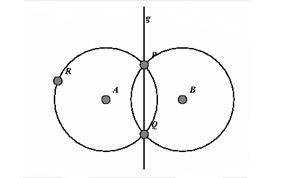
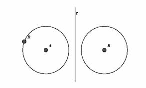
Figure 1a shows the construction of the perpendicular bisector g = PQ of segment AB by two circles of equal radius r. When dragging A, the intersection points P and Q of the circles will vanish for d (A, B) > r. However, "Cinderella" leaves g in its place (Figure 1b)!
|
|
|
|
|
Fig. 1a |
Fig. 1b |
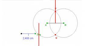
Example 2
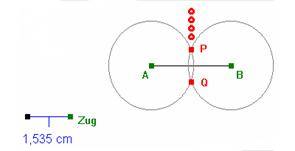
Dragging Zug changes the radius of the circle, Fig.2a. Thereby, students shall discover that the perpendicular bisector is the locus of equidistance to A and B. However, when students draw the locus of P by dragging Zug, the "Euklid" version of the interactive worksheet shows a surprising jump, Fig. 2b
|
|
|
|
|
Fig. 2a |
Fig. 2b |
Example 3
In a later stage, students shall discover the circumcentre by observing the behaviour of the intersection point P of two perpendicular bisectors. In trying this with "Cinderella", it is firstly annoying that one cannot trace the movement of P when dragging A freely – instead, one has to draw the locus of P when A varies along a curve, for instance a circle. But then it is confusing (if not misleading!) that the drawn locus is the whole perpendicular bisector - whereas dragging A reveals that P covers only a small part of it; Fig. 3.
 |
|
Fig. 3 |
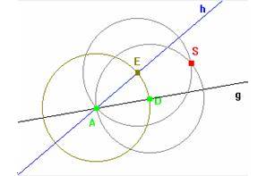
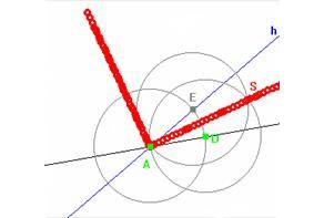
Example 4
In order that students come to know the angular bisector as equidistant locus of the two sides, they shall vary the radius in the three-circle-construction by dragging D (figure 4a). However, when D passes through the vertex, S deviates orthogonally from the expected path, as is shown by the locus of D in Figure 4b. ("Euklid", "Cabri").
|
|
|
|
|
Fig. 4a |
Fig. 4b |
Example 5
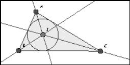
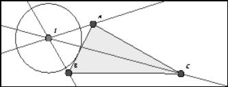
In Figure 5a, by dragging the vertices of the triangle students may discover that its angular bisectors meet inevitably in one point I. However, it may be considered harmful (especially with regard to the interpretation of I as incentre), that dragging vertex B through A lets “Cinderella” move I out of the triangle.
|
|
|
|
Fig. 5a |
Fig. 5b |
The list of examples may well be continued. Especially the last one, which occurred in classroom during an empirical study, is apt to put the teacher into real difficulties (in the observed situation, these where “solved” by reloading the worksheet). Of course, one is driven to the Question: Are these contra-intuitive effects due to
flaws of the software?
flaws of the construction?
flaws of our notions?
The latter turns out to be the case in some important aspects! This fact underlines strongly the necessity for a theory of dynamic geometry.
2 On principles of Dynamic Geometry
The unwanted behaviour of intersection points in our examples suggests to postulate the
Continuity Principle: DGS should move objects continuously in drag mode.
Also, pitfalls like the “extra triangular” incentre prompt the demand for the
Determinism Principle: For any position of the base points there should be only one position of the constructed elements.
So, why not just stick to a DGS that conforms to these principles? But unfortunately these desirable principles are mutually exclusive! In fact, we shall later prove the
Exclusion Theorem: A continuous DGS cannot be deterministic.
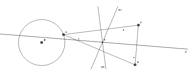
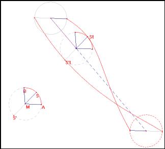
The basic example (see also Figure 6 below) illustrating this embarrassing conclusion was already mentioned by Kortenkamp (1999): Consider the angular bisector w of Ð AMB when A moves round M along k. After a full turn, the new w coincides with the original one – but with reversed orientation. This causes a problem: let w intersect k in S and S’. When B reaches A, S and S’ must
either return to their original position – in this case they behave
discontinuously!
or remain where they are – which implies that the DGS is not
deterministic!
We will make this plausible reasoning precise by the theoretical framework of section III. Meanwhile some thoughts about the didactical implications of the exclusion theorem are in order: Of course it necessitates most careful reflections on when to use what kind of DGS in order to minimise the unwanted, but unavoidable side effects of violating one of the principles. However, switching between the two worlds without comment may also cause problems for the students, since what is true for one DGS does not hold for the others.
So one may even think of deciding once and forever between the principles and confine oneself to the less harmful one. And though at first sight, continuity looks more promising, one may well be tempted to ban it from the classroom, having in mind the possibly disastrous after-effects of Example 5 on students’ understanding. Well – but the matter is even more intricate: When considering locus problems one may want the incentre to move out of the triangle for good reasons (Section IV). Thereby we arrive at
Moral 1: Further and deeper didactical considerations are necessary – especially with regard to what we really want to teach as Dynamic Geometry.
In support of this, a more solid theoretical mathematical framework may be appropriate. Therefore we sketch the following attempt:
3 Towards a theory of Dynamic Geometry
Usually, a figure F is conceived as set of points in the Euclidean plane E. Dragging a base point along a curve C amounts mathematically to traversing a parameterisation g: [0, a]®E of C. By virtue of the construction of F, the DGS then produces a family Ft of figures, where t Î [0, a] denotes time. The entirety of the dragged figures is comprised to a new entity, the drag-figure F, by the following construction
![]()
In F, the individual figures Ft are arranged like slides in a projector. The dragging process corresponds to passing through them. Mathematically this is described by projecting the dragged figures Ft to the time parameter t, i. e. the fibration p: F→I; (t, x)®t.
Now we can formalise our principles:
Definition 1: A DGS is deterministic iff for every figure F and every drag path g: [0, a]®E it fulfils
![]()
Terminological Remarks
This notion was introduced by Kortenkamp in 1999, but altered by Richter-Gebert and Kortenkamp in 2001.Nowadays they seem to have no word for the original meaning.
J.-M. Laborde (1999) calls the same property conservative. Kortenkamp (1999) and Richter-Gebert and Kortenkamp (2001) give other definitions for this notion.
Corollary: In the deterministic case one can associate to each point C of the curve C a unique dragged figure: FC: = Fg(t) for one (and thus per definitional all) tÎg-1(C)). Therefore, the time-dependent drag-figure F can be lifted to a position-dependent drag-figure F by
![]()
Definition 2: A DGS is continuous iff for every figure F and every drag path g the drag-figure F is defined by equations that depend continuously on t.
As an application of these notions, we can now give the following simple
Proof of the exclusion theorem: Consider the drag-figure of the segment F = SS’ in Fig. 6. Because S2p must be either S or S’, we have F0 = F2p and can thus form F – which turns out to be a Möbius strip. But the map t®St yields a continuous section of F that cannot be lifted to F – for otherwise the Möbius strip would be orientable, which is surely not the case. So the figure S has no position-dependent drag-figure S, q.e.d.
|
|
|
|
|
Fig. 6 |
|
4 Advanced examples – The dynamic interplay between geometry and algebra
Locus problems are a powerful realm for developing strategies and deepening the understanding of fundamental ideas. An important one is surely the Cartesian Correspondence between curves and their equations. It can be explored by a profitable interplay of CAS and DGS: By use of DGS, students can produce and investigate interesting curves and geometric loci. Thoughtful dragging may well give rise to some fairly non-obvious conjectures. The algorithms of algebra and calculus to verify them are now easily accessible by CAS. Nevertheless, often it turns out that real concordance between geometric phenomena and algebraic computations is obtained only after a thoughtful reconsideration of fundamental notions. This however should be considered not as a bug, but as a feature! The thereby attainable deepening of conceptual understanding seems most promising especially for teacher education (notwithstanding the necessity of some software debugging as well.)
Example I
Warneke (2001) has investigated the locus of the incentre I of an isosceles triangle ABC, when C moves on a circle through B centred at A. The straightforward way of constructing the locus I yields seemingly a curve with a cusp (Fig. 7a). But with elementary trigonometry one obtains a parametric representation for I and that can be transformed to an equation by some algebraic yoga based on Pythagoras’ theorem. This equation, however, turns out to describe a strophoid – and the strophoid is known to have a node as singular point! What’s going on? Some curve plotting reveals that the geometric locus is only the “inner part” of the curve that is described by either the parametrization or the equation. Warneke proposed an ingenious argument to support an alternative geometric construction of the complete locus:
The line BC changes its orientation after a full turn of C through k, so one should rather consider the angle between BC and AC. Some fiddling with the particularities of “Cabri” resp. “Euklid” is necessary in order to produce the complete locus after two turns.
So one is tempted to conclude that the continuous behaviour of “Cinderella” is didactically favourable in this case as it allows to produce the complete locus without extra effort (Fig. 7b). But the price one has to pay for this is to accept that then I moves out of the triangle ABC in every second pass of C through k.
|
|
|
|
Fig. 7a |
Fig. 7b |
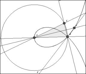
So one has:
|
either |
to refrain from using this interesting example |
|
or |
one has to give up the idea of the Cartesian Correspondence at least in its naive version (it follows from the theory of elliptic curves that the geometric locus cannot be described by an equation at all!) |
|
or |
one has to find an explanation for the “extratriangular” incentre (which may imply to re-interpret the whole story as taking place on a Riemann surface, as Gawlick (2001a) points out. |
|
if |
one not just chooses to ignore the occurring discrepancies – this alternative should of course be excluded as utterly unmathematical! |
Moral 2: To cope with interesting phenomena one has to develop dynamic notions for dynamic geometry.
Example O It is known that the locus O of the orthocentre O of a triangle ABC inscribed in an circle k is a circle, when C varies on k is again a circle, namely k reflected by AB. In order to elucidate the peculiarity of this fact Hölzl (1999) has proposed to untie B from k. A variety of interesting curves arises, of which Fig. 8 depicts only a few. One is then interested to survey them and their properties, for instance by means of an equation.
|
|
|
|
|
|
Fig. 8 |
|
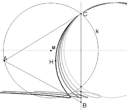
After an appropriate choice of coordinates, O is easily obtained by elementary analytic geometry, thus yielding a parametrization of O. This can be transformed into an equation by straightforward calculations, compare Gawlick (2001b). But some discrepancies occur: The equation is of degree four, so a generic line will intersect the curve in four points. However, on the screen any line hits the locus in at most three points! Is there a hidden linear factor? Yes, as one may want to check by CAS. So this was just a case of miscalculation? Yes, but probably one with probably deeper-lying reasons: one finds to one’s embarrassment that even CAS is unable to produce the correct equation for O out of the parametrization by
built-in algorithms for implicization,
resultant calculation,
Gröbner-base computation.
Most ironically, “Cabri” is able to find the equation for the curve containing the locus (again properly) by guessing (i.e. by interpolation of many random point on O)!
Moral 3: In dynamic situations, we have also to refine (our understanding of) algebraic notions in order to handle parametric equations correctly!
References
Elschenbroich, H.-J. (2001) Electronic Interactive Worksheets. Proc. of Cabri-World, Montreal.
Gawlick, Th. (2001a) Zur mathematischen Modellierung des dynamischen Zeichenblatts, in: Elschenbroich, H.-J., Gawlick, Th., Henn, H.-W. (ed.) Zeichnung - Figur - Zugfigur. Mathematische und didaktische Aspekte Dynamischer Geometrie-Software. Franzbecker, Hildesheim.
Gawlick, Th. (2001b) Exploration reell algebraischer Kurven mit DGS und CAS. Elschenbroich, H.-J., Gawlick, Th., Henn, H.-W. (ed.) Zeichnung - Figur - Zugfigur. Mathematische und didaktische Aspekte Dynamischer Geometrie-Software. Franzbecker, Hildesheim.
Kortenkamp, U. (1999) Foundations of Dynamic Geometry. Dissertation, ETH Zürich.
Kortenkamp, U.; Richter-Gebert, J. (2001) Grundlagen dynamischer Geometrie. Elschenbroich, H.-J., Gawlick, Th., Henn, H.-W. (ed.) Zeichnung - Figur - Zugfigur. Mathematische und didaktische Aspekte Dynamischer Geometrie-Software. Franzbecker, Hildesheim.
Laborde J.-M.(1999) Some Issues raised by the Development of Implemented Dynamic Geometry as with Cabri-géomètre. Proc. 15th European Workshop on Computational Geometry. INRIA.
Warneke, K. (2001) Mit DGS zu Algebraischen Kurven. MNU 54(2), 81-83.
Self-correction in algebraic algorithms with the use of educational software:
An experimental work with 13-15 years old pupils
Michalis Kourkoulos and M.-A. Keyling
Heraklion, Crete, Strasbourg, France
4. Treatment of first degree equations with whole classes
5. Results of experimental and comparison classes
6. Working with smaller groups of average and weak pupils
1 Background
Although, at present, there is not a large number of didactical researches concerning self-correction activities, the existing ones point out clearly that these activities are very fruitful for the learning of the examined subjects (see Pluvinage F., 1983, Regnier 1983, Kourkoulos 1997)
Concerning the algorithms of arithmetic and of elementary algebra, self-correction appears as a complex activity. Pupils, in order to find and to correct by themselves the errors of an exercise, need to dispose and to activate global and local[1] control criteria. In addition, they have to develop an errors’ localization strategy. Furthermore, when an error is found, they need to formulate alternative propositions and to control their correctness. (Kourkoulos 1998)
During self-correction activities pupils often activate and associate information contained in their new and previous knowledge. Moreover, in many cases they associate information from different areas of their knowledge (the pieces of information come from different conceptual frameworks -Douady R. 1984 - and /or their comparison need an interplay between different semiotic registers -Duval R. 1995). The comparison of the associated pieces of information, often, leads pupils to detect contradictions and to abort wrong ideas. In other cases, the correlation of these pieces of information help pupils to clarify the different aspects of the examined subject. (Kourkoulos 1998)
Despite the fertility of self-correction activities, often they are complex enough and without the appropriate guidance of the teachers the ability of self-correction remains limited only to the good pupils. A characteristic element on this matter is the following:
In a sample that we have examined, of 215 pupils of "B' Gymnasiou"[2] in Heraklion Crete, we found out that at the end of traditional teaching of first degree equations less than one third of the pupils was able to found and to correct their errors by themselves. Concerning the arithmetic expressions which involve positive and negative powers, the same holds for about 20% of the sample. (Kourkoulos 1997)
In these cases, the organisation and the introduction of appropriate self-correction schemes during the teaching process constitute a decisive factor for the success of the average and weak pupils (Kourkoulos 1998)
Nevertheless, the absence of organised work on self-correction is easily seen in the actual conditions of mathematics teaching, at least in the cases of Greece and of France that we have examined. (Kourkoulos 1997, 2000a Kourkoulos and Keyling to appears)
For six years, in France and in Greece, we have experimented with self-correction activities in different subjects (positive and negative numbers and priorities of operations, literal calculation, resolution of equations). The analysis of the pupils’ behaviour points out that there are some fundamental aspects which are common in the self-correction procedures of the different algorithms of arithmetic and of elementary algebra. Taking under consideration these aspects is essential for the teaching, if we want pupils to become able to control the algorithms taught and to correct their errors.
The notion of double control introduced by F. Pluvinage (1983) and the notion of the semiotic registers of representation and treatment (registres sémiotiques de représentation et de traitement) of R. Duval (1995), help us significantly to understand the way pupils use control criteria. The analysis of G. Brousseau (e.g. Brousseau 2000), was also very useful for the clarification of the role played by the learning cost and the role played by the application cost of control criteria. Our research points out that these factors are essential in the construction of pupils’ control and self-correction systems. (See Kourkoulos 1998, Kourkoulos and Tzanakis 2000)
2 Errors’ localisation
The localisation of the errors is another factor which is revealed important for the success of pupils in self-correction activities. A characteristic element indicating the importance of this factor is the following: When we decrease the difficulty of the localisation of the errors, by indicating to pupils a more restricted region of the exercise (e.g. a line of the solution procedure of the exercise) at which they have to search for the errors, a great number of those who could not do it before, succeed to find and to correct their errors.
For the self-correction activities that we have experimented, an essential element of the help offered to the pupils was to indicate them more or less restricted regions of the exercise (some lines, one line, a part of a line) at which they have to search for the errors. The width of the indicated regions was adapted to the characteristics of the pupils. These regions had to be restricted enough so that they arrive at finding and correcting their errors and large enough so that their research is difficult enough to urge them to develop their strategies for the localization and correction of the errors.
This type of help has permitted to an important number of average and weak pupils to find and to correct their errors, and in this way to get involved into the self-correction game from which they had been excluded until then, at least for the examined algorithms.
Following the improvement of their strategies of localization and of correction of errors, we were increasing the size of the regions indicated, until they were able to look for their errors in the whole exercise.
3 The software Arithm
Taking into account the aforementioned analysis of pupils’ work we were led to construct a software («Arithm»), which aims at facilitating the self-correction work of the pupils. The software function in the following way :
The pupil writes on the computer line by line the solution of his exercise, as he would do on his note book. For every line, the software indicates to him whether it is correct or not. After this, it is the pupil’s responsibility to find and to correct his error(s).
Our observations have pointed out that for an important number of
average and weak pupils one line was already a very extended region in order to
arrive at finding and correcting their errors, at least at the beginning of the
self-correction work. For these pupils, the teacher can regulate the software
in order to allow them to use the «help of extract». Using this help the pupil
can extract a part of a line and check the transformation of this part. (Every
time that the pupil proposes a transformation of the extract, the software
informs him whether this transformation is correct or not.) Besides, the
software indicate to the pupil that the part extract should not be, when the
rules of priorities have not been respected (e.g. If pupil has the line 2x
+ 3x(x-2)2 + 4x2 and he extracts 2x + 3x)
After working for some time, there are pupils who have less need of
help. In these cases teacher can regulate the software to function in the mode
of «reduced help», so that pupils’ research conserve a degree of difficulty
which urge them to develop their strategies concerning the localization and the
correction of the errors. In this mode the «help of extract» is forbidden and
the software does not give indications
of correctness for every line of the treatment. It gives indications only for
lines that the pupil asks for. Further more, a points game encourage the pupil
not to ask unnecessary help.
Other types of help can be offered to the pupils by the software (calculator of arithmetic expressions, explanatory texts, treatment of polynomial expressions). The access to this type of help is also determine by the teacher. Furthermore, the teacher can define an automatic increase of the level of the help offered in case that pupil fails repeatedly to find and to correct the errors of a region.
The software records in detail pupil’s work. Besides this, it can provide some statistical measures for that record (these measures are very useful to the teachers, because they permit them to have a rapid, but global, view of pupils’ work). The software proposes exercises chosen by the teacher. It can treat exercises from its library, from electronic sheets constructed by the teacher or exercises which pupils copy directly from the blackboard. So it offers to the teacher the possibility to propose at the different categories of pupils different group of exercises, according to their characteristics. ( See also Keyling et al : L’emploi du logiciel «Arithm» en classe, to appear, IREM of Strasbourg)
4 Treatment of first degree equations with whole classes
Using this software, teachers alone in their class was able to realise the self-correction activities we proposed:
With 3 experimental classes and 4 comparison classes, of B' Gymnasiou, we have realised a teaching in which 1st degree equations was introduced and treated. The duration of teaching was 22 hours for each class. In meetings preceding teaching we have informed the teachers of the 7 classes on the results and the methods emerging from didactical studies concerning 1st degree equations (Vergnaud G.,1990, Filloy E. and Rosano T.,1985, Kieran C.,1990). In addition, we have informed them on the results of didactical researches concerning control and self correction activities (Pluvinage F, 1983, Duval R,1995, Regnier J.C,1983, Kourkoulos M et al ,1998, 2000b)
The difference between experimental classes and comparison classes was that the first spent 8-9 (of the 22) hours on self-correction activities using «Arithm», while the second spent 4-6 hours in self-correction activities without the use of computer.
Self-correction activities in comparison classes was based on traditional arithmetic verification and local control criteria taught by the teachers. Verification was also used in the intermediate equalities of the solution[3].
Although it was initially planned to spend about 8 hours on self-correction activities based on arithmetic verification, the teachers of comparison classes preferred to spend less time with these activities because they have the feeling that : concerning the more complex types of equations (see type 2 and 3 below) arithmetic verification was less efficient for average and weak pupils who have difficulties and commit frequent errors in the calculation of arithmetic expressions. On the one hand, for these pupils verification becomes a long duration and uncertain control procedure and on the other hand, teachers being alone in their classes, could not offer the necessary individual help to the pupils who needed it. So they prefer to spend more time on traditional training on equations solution (solution with teacher’s assistance and correction to the blackboard).
In all classes teaching was realised at three levels:
simple equations, up to the equations having more than one occurrence
of x in both sides and containing only integer coefficients and constants (e.g.
3x - 5x + 11 = 9x + 17 + 3x)
equations containing brackets and integers, up to the equations
having more than one occurrence of x
in both sides (e.g. 3x - 5(2x-3) = 4x + 3(6-x) - 10)
equations containing fractions, up to the equations containing sums
to the numerators
![]()
In experimental classes the following scheme was applied for each level:
Lecture and initial practice’s applications (without computer) in
order to introduce the necessary elements
for the treatment of the examined equations (algorithms of solution, interpretative models, control
criteria).
Self-correction activities in which pupils work with «Arithm».
During these activities, most pupils were arriving at finding and correcting
their errors by themselves (without teachers’ help). This allowed teachers to
have more available time to give individual help to average and weak pupils who
could not find or correct their errors despite of the help provided by the
software. To these pupils teachers were reminding or explaining local control
criteria and the way to realise the different tasks. In certain cases, looking
at the behaviour of these pupils, teachers were led to give new explanations or
control criteria that they had not taught previously in the class.
At the end of self-correction activities with «Arithm», teachers
prepared and performed teaching containing complementary explanations, control
criteria and algorithm’s modifications concerning the difficulties and the
errors that pupils do not arrive to overcome during self-correction activities.
A part of these explanations, control criteria and algorithm’s modifications
was recently formed by the teachers. Teachers were led to form these elements
because of the detailed observations of pupils behaviour. (The fact that
teachers make more detailed observations than they usually do, result, on the one hand from the fact that the
software permits them to spend enough time to individual observation and
intervention concerning average and weak pupils and on the other hand, from the
exploitation of the detailed record of the pupils’ activities provided by the
software).
After the complementary courses of the second and of the third part
of the teaching, teachers devoted another one or two hours on self-correction
activities with «Arithm».
In the three experimental classes 8, 9, 10 hours were devoted respectively in introductory courses, 9, 9, 8 hours in self-correction activities with «Arithm»( first and second period) and 5, 4, 4 hours in complementary courses.
During the teaching period, the teachers of experimental classes remarked that it would be useful for many average and weak pupils to spend more time on self-correction activities with «Arithm», in order to make further progress on the examined subjects. So they asked a prolongation of self-correction activities. However this was not done, in order that the teaching time of the subject in experimental classes would not be significantly longer than that available in the comparison classes or in the usual classes at this level (B’ Gymnasiou).
5 Results of experimental and comparison classes
In the questionnaire given before the teaching activities, the results of experimental and comparison classes are equivalent. It is characteristic that for the equations 5x = 8, 3x-6 = 20, (5/7)x = 11, (x+2)/5 = 7 find respectively the correct solution: 43%, 28%, 17%, 23% of the pupils in the experimental classes and 45%, 26%, 15%, 24% of the pupils in the comparison classes.
At that moment pupils consider these equations as problems of practical arithmetic («Find the number which...»). Nevertheless, the knowledge and the abilities necessary for their solution are important for the understanding of the algebraic algorithms used to solve 1st degree equations (understanding the problem posed by an equation, inversion of operations, operations and properties of fractions, priorities of operations).
In the final questionnaire, given three months after the end of the teaching, the differences between the results of experimental and of comparison classes are statistically significant for all the examined questions (level of significance 5% or smaller).
For the simple equations (5x = 8, 3x-6 = 20, 2x-25 = 5x+10) find respectively the correct solution: 87%, 83%, 75% of the pupils in the experimental classes and 74%, 67% , 61% of the pupils in the comparison classes. For the equation with brackets: 8 + 2(5x+4) = 15x + 13 and the simple equations with fractions:
![]()
find respectively the correct solution: 76%, 72%, 73% of the pupils in the experimental classes and 54%, 51% , 48% of the pupils in the comparison classes. On more complex equations containing fractions
![]()
find the correct solutions, respectively: 61%, 52% of the pupils in the experimental classes and 36%, 24% of the pupils in the comparison classes.
We observe that the difference of success between experimental and comparison classes is 13% -16% for simple equations but when the equations become more complex it increases, up to 25% and 28% for the equations with many fractions. This fact is related to the improvement of error’s localization strategies, which is much greater for the pupils of the experimental classes. The role of these strategies in self-correction is more important when the exercises are more complex. (see also Kourkoulos 1997).
6 Working with smaller groups of average and weak pupils
At Strasbourg we have chosen to explore self-correction activities with the use of «Arithm» working with smaller groups of pupils (7-12), in the framework of «supportive teaching» («enseignement de soutien» ), in order to be able to observe pupils behavior more profoundly. With one exception, these groups was constituted by average and/or weak pupils.
During two years we have been working with 6 groups of «4ème», on the arithmetic operations with positive and negative numbers and the priority of operations in arithmetic expressions. The duration of group’s work on these subject was 4-6 meetings. In one group two good pupils have participated, the 10 other members of this group were average and weak pupils. The other groups were constituted by average and weak pupils (2 groups) or by weak pupils (3 groups).
The first group of 4ème have also worked on the development and the reduction of polynomial expression, during 4 meetings. We have worked on the same subject with two groups of weak pupils of 3ème during 8 meetings and with one group of average and weak pupils of 3ème during 6 meetings.
The results of the experimental work in France converge with those of the experimental work in Greece and they permit to point out some essential elements concerning self-correction and the learning of the algorithms examined:
The question of the localisation of the errors appears strongly related to pupils’ capacity to decompose an application of an algorithm in units of calculation, that is in expressions which can be treated and controlled independently. This subject presents important difficulties for a considerable number of average and weak pupils. At the beginning of the experimental work, some of these pupils effect such a decomposition work but the decompositions they do are often wrong since they do not respect the priorities of operations (e.g. A pupil has transformed one line of the algorithm: 2x + 4x - 9x(x+1)2 + 6x + 11x to the following: -3x(x+1)2 + 17x and tried to control if 2x+4x-9x is equal -3x). Others consider the transformation from one line to the next only as a transformation of the whole line and make no decomposition at all, even in cases that their transformation contains many and/or complex steps. Besides, some time after the end of a transformation, many of these pupils are not able to identify the steps that they have done in order to realise these transformation.
Despite of the work realised with self-correction activities, a part
of these pupils don’t succeed to overcame these difficulties. These pupils
cannot decompose their own written work (applications of algorithms) in units
of calculation which can be treated and
controlled independently. This ability is directly related to the ability to
consider an algebraic expression as composed from computational units related
among them with the rules of priority.
So it is an ability having a fundamental character for the learning of algebra.
At the end of experimental work, these pupils have better results in simple
exercises, containing one elementary operation (e.g. one operation with
positive and negative numbers) or containing a repetition of operations of the
same type (e.g. the sum or the product of many positive and negative numbers).
However, they do not succeed to treat correctly more complex exercises.
A second part of these pupils progresses slowly but significantly in
the decomposition of algorithms in units of calculation which can be treated and controlled independently. The
progress of these pupils depends substantially on the duration of
self-correction activities in their group. (These facts led us to increase the
duration of group’s work in the last year.) Given sufficient time to work,
these pupils present an important evolution concerning their self-correction
strategies. In addition, they present a significant improvement on the
treatment of simple and of complex exercises as well. (There are pupils in this
category who, after some time, present a very strong improvement, which
indicates an unblocking in the understanding of the significance and the
organisation of algebraic expressions.)
Another part of pupils do not have important difficulties to
decompose an algebraic expression in units of calculation which can be treated independently but they have not
incorporated this type of work in their error’s localisation procedures. These
pupils realise important progress even when they work for a relatively short
period with «Arithm» (4-5 hours): They learn to use in a systematic way the
decomposition of the transformations done in units of calculation which can be
controlled independently in order to locate their errors. This provokes a
significant improvement of their self-correction procedures. In addition, they
present an important amelioration concerning the treatment of simple exercises
and an even more important one concerning the complexes exercises of the
examined subjects.
An other element to be noted is that the learning achieved in the treatment of one subject (e.g. treatment of arithmetic expressions) concerning the separation of the algorithms in independent units of calculation and the localisation of the errors, is transferred and reinvested on the treatment of others subjects (e.g. literal calculation, resolution of equations of 1st degree).
In addition, both in Greece and in France, we have observed the same type of changes in the general behaviour of pupils concerning the subject of self-correction: They consider control and self-correction as very useful, they search and ask for control criteria and self-correction procedures in traditional teaching of the subjects which have been treated after the experimental work.
References
Adam L., Meirieu Ph., Richarde Ch. (1986) Différencier la Pédagogie (Français-Mathématique). C.R.D.P. Lyon.
Brousseau G. (2000) Les propriétés didactiques de la géométrie élémentaire. Acts of 2th C.D.M. Ed. Univ. of Crete, 67-83.
Douady, R. (1984) Le jeux des cadres. Doctorat, Université Paris VII
Duval, R. (1995) Semiosis et pensée humaine. Ed. Péter Lang, Berne.
Filloy, E., Rosano. T., (1985) Obstructions on the acquisition of elementary algebraic concepts and teaching strategies. P.M.E., 134 – 147.
Keyling e.a., (2002) L'emploi du logiciel "Arithm" en classe. IREM de Strasbourg.
Kieran C. (1981) Concepts associated with the equality symbol. Educational Studies of Mathematics 12, 317-326.
Kieran, C. (1990) Introducing Algebra: A functional approach in a computer environment, 14th I.C.P.M.E., Mexico, vol II, 51-59.
Kourkoulos M. (1997) Self-correction and the use of educational software in learning the algorithms of arithmetic and algebra (in Greek). Acts of the 1st Colloquium of the Informatics Teachers Society on Informatics in Education, 31-58.
Kourkoulos M. (1998) Caractéristiques des critères de contrôle utilisés par les élèves à l'application des algorithmes de l'Arithmétique et de l'Algèbre. Acts of 1st C.D.M., Ed. Univ. de Crète et Institut Français d'Athènes, 224-236.
Kourkoulos, M., Tzanakis, K. (2000) (in Greek) Estimation and checking procedures as fundamental aspects of the conception and learning of mathematics algorithms. Acts of 2nd C.D.M. Ed. Univ. de Crète, 264-285.
M. Kourkoulos, M.-A. Keyling,2000, “L'autocorrection dans l'apprentissage des algorithmes de l'algèbre élémentaire et l'emploi du logiciel Arithm”, Colloque International: “Enseignement des Mathématiques 20000” organisé par la CFEM en coopération APMEP et SMF, Grenoble, (acts to appears)
Pluvinage, F. (1983) Variations des questions, questionnaires à modalités. Acts of 4th I.C.M.E., Berkley, 465-477.
Regnier, J.C. (1983) Etude didactique des tests autocorrectifs en trigonométrie. Thèse de doctorat, U.L.P.
Vergnaud, G., Cortez A. (1990) From arithmetic to algebra: Negotiating a jump to learning process. Proc. of 14th I.C.P.M.E., Mexico, vol 2, 27-35.
A CAS-index applied to
engineering mathematics papers
Eoghan MacAogáin
Limerick, Ireland
4. Analysis of MA4002 Engineering Maths 2 - Spring 2000, Univ. of Limerick
5. Calculation of the CAS-index for papers MA4002/MA4001
6. Examples of questions in the various categories
A CAS-index is applied to a set of first year university engineering mathematics examination papers; the results are analysed. The CAS-index is an index of suitability. Its purpose is to try to answer the following question: given a mathematics examination paper which was written for a CAS-free environment how is the level of difficulty of that paper affected when it is answered with the aid of CAS?
1 Two classifications
Traditional mathematics examination papers assume that students do not have access to symbolic manipulation systems. Several people have investigated what happens when we use CAS to help answer a traditional mathematics examination paper. One approach is to classify the questions according to the impact, which CAS has on them. We’ll describe two such classifications (others have been proposed by Kokol-Voljc and Kutzler).
Jones (1995) offers the following categories:
1 No impact: because the graphics calculator contributes little or no more to the completion of the task than a scientific calculator.
2 Impacts: by providing alternative, but mathematically valid, methods of solution.
3 Trivialises: by providing alternative methods of solution that require little or no mathematical input from the user.
I use the following classification; it is rather similar to the Jones classification but is based solely on how the use of CAS affects the level of difficulty of the question:
CAS-proof: the use of CAS does
not affect the level of difficulty of the question; CAS does not help the
student to answer the question, or only very marginally.
Slightly easier with CAS:
question becomes slightly easier when CAS is used.
Significantly easier with CAS:
question becomes significantly easier when CAS is used.
Trivial with CAS: with the use
of CAS the question becomes trivial.
2 Weighting
In the above classifications there is a certain gradation in the categories. For example, in the last classification the categories range from less impact to more impact on the level of difficulty of the question. Some natural questions to ask are: What would be the effect if we attached various weights to the categories? Can we discover anything by so doing? Can we develop useful measures? What information could such measures give us? In particular we wish to ask which questions are still suitable in a CAS-supported environment. Plainly, those in the “trivial with CAS” category are no longer suitable. Those in the “significantly easier with CAS” category also need to be changed. We could argue that questions in the other two categories are still suitable in a CAS-supported environment. Let us apply the above ideas by attaching weights to the categories as follows:
|
Category |
Weight |
|
CAS-proof Slightly easier with CAS Significantly easier with CAS Trivial with CAS |
1 1 0 0 |
3 A CAS-index
We wish to come up with a single number, which will give a measure of how suitable a particular examination paper is for use in a CAS-supported environment. The rubric of the examination paper, for example, “answer four questions out of six”, is an important factor. Students will generally answer what they see as the easiest questions. If the rubric says “answer all questions”, we can simply apply our weights and essentially calculate what proportion of questions are suitable. However if a student has a choice of which questions to answer the situation is slightly more complicated. To arrive at our measure we ask the following question: “What score would a student get by correctly answering questions in the two unsuitable categories?“ If this number is high the examination is unsuitable; if the number is low the examination is still suitable in a CAS-supported environment.
We calculate the CAS-index as follows: let x% = student’s score obtained by correctly answering all questions in the categories “trivial with CAS” and “significantly easier with CAS” (taking the rubric of the examination into account); calculate (100-x)/10 (rounded to an integer); range of index: 0-10; interpretation: 0: unsuitable in a CAS-supported environment; 10: suitable in a CAS-supported environment.
4 Analysis of MA4002 Engineering Maths 2 -
Spring 2000, Univ. of Limerick
Table: Score answering trivial or significantly easier questions
|
Question |
1 |
2 |
3 |
4 |
5 |
6 |
7 |
|||||||||||||||||||||
|
With CAS: |
a |
b |
c |
d |
e |
f |
g |
h |
i |
j |
a |
b |
c |
a |
b |
c |
d |
a |
b |
c |
a |
b |
c |
a |
b |
c |
a |
b |
|
Proof |
|
|
|
* |
|
|
|
|
|
|
|
|
|
|
|
|
|
* |
|
|
* |
* |
* |
|
|
|
|
|
|
Slightly easier |
* |
|
|
|
|
½ |
½ |
|
* |
|
|
|
|
½ |
½ |
½ |
½ |
|
* |
* |
|
|
|
* |
|
* |
|
|
|
Significantly easier |
|
* |
|
|
* |
½ |
½ |
* |
|
|
|
|
|
½ |
½ |
½ |
½ |
|
|
|
|
|
|
|
* |
|
|
|
|
Trivial |
|
|
* |
|
|
|
|
|
|
* |
* |
* |
* |
|
|
|
|
|
|
|
|
|
|
|
|
|
* |
* |
|
Score |
24 |
20 |
10 |
0 |
0 |
4 |
20 |
|||||||||||||||||||||
5 Calculation of the CAS-index for papers MA4002/MA4001
The CAS-index was calculated for two first-year engineering mathematics papers of the University of Limerick. The CAS used was Derive. We’ll examine MA4002 in detail. Its rubric is as follows: “Answer question 1 and any other three questions …”. The marks available are: question 1: 40, each other question: 20, maximum: 100.
Choosing questions 1, 2, 3 and 7 the student obtains a mark of 74% by correctly answering the sections in the two unsuitable categories. x = 74. (100 – x)/10 = (100 – 74)/10 = 2.6 which rounds to a score of 3 on the CAS-index. Interpretation: this paper would be unsuitable for use in a CAS-supported environment. Note that while this paper contains three suitable questions the student can avoid these because of the rubric and so the paper as a whole would be unsuitable in a CAS-supported environment (of course, it was designed to be answered without CAS).
The score on the CAS-index for the examination paper MA4001, without going into the details, works out to be 2. Interpretation: this paper would be unsuitable for use in a CAS-supported environment.
6 Examples of questions in the various categories
CAS-proof
State the Mean Value Theorem. By applying it to
f(x) = (1+x)^r-1-rx on some interval,
prove that (1+x)^r > 1+rx for all x>0, where r>1. (MA4001 q.3(a))
CAS is evidently no help in the first part of this question. In the second part, CAS could help in a small way, for example in carrying out the differentiation. Typically, if we are asked to prove a theorem or carry out an operation in a specified fashion, e.g. differentiate from first principles, then CAS is not of much assistance.
Slightly easier with CAS
A radioactive substance has a half-life of 1000 years. How much of an initial amount of the substance is remaining after 700 years? (MA4002 q.4(b))
To answer this question the student needs to have a “road-map” of the necessary procedures: write down the differential equation / solve the differential equation / apply the half-life to evaluate the constant / answer the particular question asked. While CAS helps with some of these steps, in particular with solving the differential equation, the main work is still done by the student. While CAS helps with some of the procedures the student must know what steps to take to answer the question.
Significantly easier with CAS
Find all first and second partial derivatives of
f(x, y) = 2cosh(lnx – lny)
(Hint: first simplify!). (MA4002 q.1(h))
Using CAS: enter the function / simplify / find the derivatives. CAS does most of the work, but the student still needs to understand the question, needs to interpret “all first and second partial derivatives”.
Trivial with CAS
Find the inverse of the 3x3 matrix [[1,3,-1], [3,0,2], [5,4,1]]. (MA4002 q.7(b))
Using CAS this reduces to the following procedure: enter the matrix A; evaluate A^(-1). This is typical for questions which are testing particular skills. With CAS they tend to reduce to a two-stage process: enter the expression or function / carry out the required operation, e.g. simplify or integrate. More accurately, it is a four-stage process: read the question / enter the expression / carry out the required operation / write down the answer.
7 Discussion
How valid is the CAS-index? There are obviously various factors which would affect the results:
the choice of CAS used: for
example, some CAS contain a substantial statistics package while others do not
the level at which we use the
CAS: we assume a level of knowledge of the particular CAS which a student would
have after an introductory course --- what is described by Kutzler as “Routine
CAS-Use”
the classification scheme which
is used
which categories the questions
are placed in: this part of the procedure is rather subjective; there are no
clear boundaries between the categories
the weights used for the
various categories: one might argue for a different weighting
In spite of the reservations expressed above, the proposed CAS-index yields a simple measure; when applied to particular examination papers the resulting scores seem to yield intuitively meaningful results. We are concentrating on one variable only: the level of difficulty of the paper. Could we develop other indices for other variables and end up with a vector of CAS-indices?
Appendix: Technology in 6th century Ireland
My Hand Is Weary With Writing
[Ascribed to Colum Cille, 521 - 597 A.D.; translated from Irish by Gerard Murphy]
My hand is weary with writing; my sharp great point is not thick; my slender-beaked pen juts forth a beetle-hued draught of bright ink.
A steady stream of wisdom springs from my well-coloured neat fair hand; on the page it pours its draught of ink of the green-skinned holly.
I send my little dripping pen unceasingly over an assemblage of books of great beauty, to enrich the possessions of men of art --- whence my hand is weary with writing.
References
Jones, P. (1995) Graphics Calculators in Traditional Year 12 Mathematics Testing. Proceedings of the 15th Biennial Conference of the AAMT, 221-227.
Kokol-Voljc, V. (2000) Exam Questions when using CAS for School Mathematics Teaching. International Journal of Computer Algebra in Mathematics Education 7(1), 63-76.
MacAogáin, E. (2000) Assessment in the CAS age: an Irish perspective, Exam Questions & Basic Skills in Technology-Supported Mathematics Teaching, Proceedings Portoroz 2000, 141-144.
Improving maths skills with CAS technology
A CAS project carried out in Scotland
with 16-17 year olds using TI-92s
Tom Macintyre
Edinburgh, Scotland
The role of Computer Algebra Systems (CAS) in school mathematics is currently being debated, with a prime focus on how this technology can be accommodated within the existing assessment frameworks. Wilfried Herget et al (2000) stimulated this debate through their article on Indispensable manual calculation skills in the CAS environment by proposing assessments are undertaken in two parts – a calculator free section and another part in which all kinds of technology, including CAS, may be used. Gardner (2001) published a reaction to this starter paper, with a somewhat provocative title of Education or CAStration? This article prompted other thoughts on what CAS brings to the classroom. The outcomes of this project in Scotland are a lot more positive than that portrayed by Gardner – favouring the terms motivation, interpretation and appreciation over CAStration; all leading the students to a fuller understanding and hopefully a better education in the process.
The study was based on research evidence gathered from students and teachers in six secondary comprehensive schools in Scotland. Three schools were treated as the study group, and three paired-control schools were identified on publicly available data. Year-12 students were targeted as they prepared for their Mathematics (Higher) course examined by the Scottish Qualifications Authority (SQA). The research sought to ascertain the potential benefits and problems of using hand-held CAS in the teaching and learning of mathematics and to identify what ways, if any, the curriculum and associated assessment in Scotland might need to change in the light of CAS tools.
During their one-year programme the students in the study group were all issued with hand-held CAS technology, allowing dedicated access to be achieved in school and at home. There is currently a ban on the use of CAS technology in any SQA assessment so the staff and students focused their attention on the learning process. Separating the learning from assessment was essential in this study and provided the opportunity to assess the impact that CAS technology had on maths skills, in particular the students’ algebraic abilities. Monaghan (2001) picks up on the need to separate these issues, acknowledging that students and teachers do a great deal in learning and teaching that is not directly related to assessment. With that in mind, the support materials provided by the researchers highlighted the ways that CAS might be utilised in the learning process. A feature of the teachers’ notes was the emphasis on the different possibilities with the calculator, in the way it might be used as a White-Box (WB) or a Black-Box (BB) as described by Kutzler (1996). An added dimension to these approaches was to use the CAS as a Grey-Box (GB) – promoting investigative approaches in the development of concepts and aiming to remain in close contact with the mathematics involved, through constantly interpreting what was produced by a BB operation. These approaches were more transparent than any BB operation – thus the proposed nomenclature!
Evidence from studies carried out by Aarstad (1998), Schneider (1997) and Brolin & Bjork (1995) indicate that the use of CAS can support and even improve students’ ability to learn crucial algebraic ideas. An analysis of algebraic skills was therefore included in the study as a means of comparing performance across the ‘intervention’ and ‘control’ schools and between the pairs of matched schools. Algebraic topics were considered in the widest sense, catering for any manipulation and handling of generalised forms, including applications within calculus and trigonometry. The range of mathematical content that was assessed in the base line and follow up assessments is detailed in Table 1.
Table 1: Mathematical content of assessments
|
Content |
Algebraic Skills Base line |
Algebraic Skills Follow up |
|
Expansion of brackets |
• |
• |
|
Factorising expressions |
• |
• |
|
Solving equations and inequations |
• |
• |
|
Change the subject of a formula |
• |
• |
|
Working with indices |
• |
• |
|
Working with Functions |
|
• |
|
Working with surds |
• |
• |
|
Solving systems of equations |
• |
|
There is a clear overlap in the content that was assessed at either end of the one-year course. In the follow up test, some of the assessment items were repeated in exactly the same format while other new items took the content forward to a higher level, e.g. incorporating items involving surds and indices within calculus. This structure enabled an analysis of matched questions to be treated separately from new questions. The general format adopted in each section enabled the researchers to gauge the student’s ability and level of confidence within each aspect of mathematical content. Increasingly more difficult questions were presented, anticipating a threshold level at which point the student might reach a limit in that particular section e.g.
Expand 2(x+3) … to … (x2+6x+3)(x2+5x-3)
Factorise 3x+6y … to … x3-x2-x+10
Indices a2 ´ a5 … to … solving 2a ´ 2a+1 = 8
Simple … to … Complex
The second assessment did not offer such a 'lead-in' on all of the sections, challenging the students to only a couple of items that were pitched at the more complex end of the topic. The base line test accounted for 45 items, with 29 test items in the follow up test. A level of attrition was evident in the course of the year but 227 students remained in the study and provided the basis for the analyses detailed below. Although the schools were paired on publicly available data it was essential to monitor the students mathematical abilities on some common footing, thereby providing a basis for appropriate comparisons to be made. The mean performance across each school is shown in Figures 1 to 3, highlighting the match across the schools at this base line measure of performance in algebraic abilities. Each of the test items was marked out of 2 with partial credit given where there was evidence of the ability being demonstrated. It is apparent that control schools C2 and C3 are slightly stronger than their corresponding pairs in the study group; the first pair is reasonably well matched.
|
|
Fig. 1 |
|
|
Fig. 2 |
|
|
Fig. 3 |
These overall scores include the performance of the easier lead-in questions; for the subsequent analyses carried out on the matched questions and the new questions the performance in the base line matched questions was recalculated.
For each school a single measure of performance was calculated, providing an overall score at the base line stage and again after the follow up assessment. These base line performances are displayed in Table 2.
Table 2: Overall performance in base line assessment – Status I: Intervention; C: Control
|
School |
Status |
Number of Students |
Base line |
|
|
Mean |
Std. Dev. |
|||
|
1 |
I1 |
37 |
0.99 |
0.28 |
|
2 |
C1 |
68 |
0.97 |
0.31 |
|
3 |
I2 |
49 |
0.97 |
0.35 |
|
4 |
C2 |
26 |
1.08 |
0.28 |
|
5 |
I3 |
28 |
0.98 |
0.32 |
|
6 |
C3 |
19 |
1.15 |
0.36 |
|
Total |
227 |
1.00 |
0.32 |
|
The results of the follow up test show that the students found the test items harder than those attempted in the base line assessment. This is understandable when one considers the composition of the follow up assessment, with fewer lead-in questions and a clearer focus on the more demanding end of the mathematical content. The implication for the analysis is that full account needs to be taken of the base line performance and the analysis must be on a within case basis, on the longitudinal data.
Table 3 shows the performance on the matched questions in the base line and follow up assessments. The performance on the new questions is also presented in this table, which presents all the data that will form the basis of the statistical analyses that follow.
Table 2: Scores on matched questions and new questions – Status I: Intervention, C: Control
|
Status |
Number of Students |
Matched questions |
New questions |
||||
|
base line |
follow up |
follow up |
|||||
|
Mean |
s.d. |
Mean |
s.d. |
Mean |
s.d. |
||
|
I1 |
37 (3%) |
0.42 |
0.36 |
0.81 |
0.51 |
0.84 |
0.39 |
|
C1 |
68 (82%) |
0.53 |
0.37 |
0.81 |
0.44 |
0.73 |
0.42 |
|
I2 |
49 (84%) |
0.49 |
0.42 |
0.77 |
0.48 |
0.62 |
0.42 |
|
C2 |
26 (34%) |
0.64 |
0.37 |
0.79 |
0.42 |
0.72 |
0.39 |
|
I3 |
28 (62%) |
0.49 |
0.40 |
1.14 |
0.48 |
0.95 |
0.41 |
|
C3 |
19 (45%) |
0.73 |
0.41 |
1.08 |
0.61 |
0.85 |
0.54 |
|
Total |
227 (64%) |
0.53 |
0.39 |
0.86 |
0.49 |
0.76 |
0.43 |
This table draws attention to the reversal of performance in the third grouping of intervention and control, with the intervention school showing a higher level of achievement in the follow up assessment having started with a lower base line. Apart from that obvious feature the rest of the data appears to be reasonably matched when the follow up performance in scrutinised.
Although the schools were matched, it is evident from Table 3 that there was a difference in school performance at the base line stage. The schools and individual pupils are starting at different levels so this fact was accounted for in the analysis of impact that may be attributed to the intervention of CAS. Taking the base line benchmark as the students’ performance in the matched questions, scatterplots have been drawn to ascertain if there was any relationship between this level and the final performance on the matched questions. The resultant graphs are shown in Fig. 4 and 5
|
|
Scatterplot of matched questions |
|
|
|
|
|
|
|
Matched Questions (Base Level) |
|
|
|
Fig. 4: Intervention schools |
Fig. 5: Control schools |
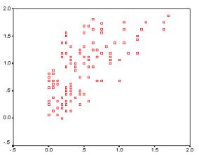
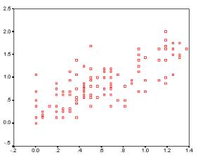
There was a strong relationship between these variables and the regression model derived through the SPSS package, demonstrated a highly significant result, with the students’ resultant performance significantly better than those from the control schools (p=0.004). The regression model takes account of the school status (intervention / control) and the base line performance in the matched questions, resulting in the following prediction for the Intervention status:
MatchedQ = 0.137+0.320+0.893BaseLineQ.
The result of taking the base line adjustment into account, is an increase of 0.137 on the overall score out of 2 [7% increase in the intervention schools]
A similar analysis carried out on the new questions, also demonstrated an increase in attainment although it was not as significant as with the matched questions. The regression model again took account of the school status and the base line performance in the matched questions. The student performance was significantly stronger in the intervention schools (p=0.046), with the model leading to the following prediction for the intervention status:
NewQ = 0.0973+0.393+0.606BaseLineQ.
The result of taking the base line adjustment into account is an increase of 0.0973 on the overall score out of 2 [5% increase in the intervention schools]
The intervention schools performed significantly better at the end of the study on the matched questions, those repeated from earlier in the year, as well as on the new questions that were of a more challenging variety. The question remains on whether this was down to the intervention of the CAS technology or other factors that may not have been accounted for. The small samples that were worked with in this ‘pilot’ study limited the strength of evidence that was generated and the non-response rate presented further limitations. Another point worth noting is the fact that some of the study group opted out of using the calculator during the year – primarily because of the assessment implications referred to below. If students could be encouraged to take up the opportunities more fully then a stronger case might be presented in favour of the CAS within the learning phase.
Questions remain on how the CAS technology contributed to the students’ learning and algebraic development. Qualitative interviews with the staff and focus group discussions with the students in the study group raised a number of issues that are worthy of following up in a more focused manner as this pilot study is extended into another academic session. The issues raised by those involved included dimensions related to the use of technology; mathematics education; and educational change in the wider context. The teaching approaches adopted by the staff had a bearing on the level of student uptake and promoted sound mathematical thinking on the part of the students. The technology focused attention on mathematical content and presentation. This took the form of mathematical equivalence, rigour and the notational forms that the students were exposed to as they used the CAS features on the calculator. Not only were they exposed to these mathematical features, but there was also an expectation and indeed a need for them to use that mathematical representation and syntax in the course of their work on the machine. The structure and rigour demanded by the CAS encouraged the students to engage with the concepts that were being tackled, but some found those demands excessive. One of the respondents claimed that ‘Some were confused and spent most of the time trying to use the calculator rather than doing the maths’; another student felt ‘you could be good at maths and not good on the calculator’. Those that did engage with the technology felt it helped them make sense of the processes and instilled greater confidence in their work. Motivation was clearly there for the students as they explored the use of the calculator in their own time and used them in other subject areas like physics. All of these opportunities increased through the dedicated access afforded to the students.
The greatest barrier to further use of CAS during the year was assessment; taking us back to the opening references at the start of this paper. Students were unwilling to use the CAS as it was designed by the researchers because it was not allowed in the examination. Staff felt under pressure of time to complete the coursework, particularly because some work had to be demonstrated using the more basic calculator technology that was permitted by the SQA; the fact that CAS and QUERTY keyboards were disallowed in the examinations limited the actual uptake during the learning process. Both staff and students had difficulties in separating learning from assessment. The fact there was no restriction on technology used in the learning phase should have meant that hand-held CAS, along with any other computer packages staff saw fit to use, should have been utilised to the full in an effort to enhance the learning taking place. This is an area that staff could promote more fully as they demonstrate appropriate use of the technology in their teaching and general work with a class, recognising that assessment can be viewed independently from the learning process. The benefits of CAS certainly appear to be there, enhancing the students’ engagement with mathematics, but in order to get the full support from the students and their parents, a clearer position needs to be stated over the direction of assessment. Some movement towards the proposal put forward by Herget et al for an examination permitting any technology would be a good start – but what will be assessed?
References
Aarstad (1997) Forsok Med Symbolsk Lommeregner TI-92. Strand Vid. Skole, a report of a pilot study in Norway, 1996/7.
Brolin & Bjork (1995) Using new technology as a tool to increase student understanding of Calculus. ICTMT 2 proceedings. Napier University.
Gardner (2001) Education or CAStration. Micromath 14.1, 6-8.
Herget, Heugl, Kutzler, and Lehmann (2000) Indispensable manual calculation skills in the CAS Environment. Micromath 13.3, 9-17.
Kutzler (1996) Improving Mathematics Teaching with DERIVE. Chartwell-Bratt, Lund.
Monaghan (2001) Reaction to Indispensable manual calculation skills in the CAS environment. Micromath 14.1, 9-11.
Integrating MuPAD
into the teaching of mathematics
Miroslaw L. Majewski and M. E. Fred Szabo
Zayed, United Arab Emirates, Montreal, Canada
2. Command-based vs. menu-based teaching
In this paper we discuss a number of proven strategies for using computer algebra to teach undergraduate mathematics, based on the extensive experience of both authors in the teaching of mathematics with technology. Although some of these strategies apply to several computer algebra systems, we concentrate on a number of the particular benefits of using MuPAD as a pedagogical tool. We consider this paper to be a contribution to the broader question of how the availability of computer algebra systems and the Opportunities inherent in the web-based information exchange can benefit the teaching and learning of mathematics in general, and of geometry and algebra, in particular.
1 Teaching with technology
Several powerful command-based mathematical packages such as Maple, Mathematica, MuPAD and others have been refined to point of providing interesting opportunities for pedagogical innovation. For Maple and MuPAD, there even exists a natural-language interface in the form Scientific Notebook, allowing us to teach and learn mathematics without the need to write and execute commands. Each approach has its advantages and disadvantages, and the authors have experimented with both methods in their teaching.
While there is an obvious affinity between traditional teaching and the natural-language electronic approach made possible with the creation of Scientific Notebook front end to MuPAD and Maple, the pedagogical advantages afforded by command-based teaching and learning are less immediate. We have therefore decided to present some of our conclusions about the benefits of the command-based approach. It is our experience that having a programming language with mathematical functions available in the classroom has at least two fundamental benefits. It can influence positively how our students think about mathematics and it improves the way in which they learn to solve mathematical problems. By using computer algebra systems, they can visualize mathematical concepts, especially certain types of functions and equations, they can solve realistic problems without the need for tedious calculations, and can manipulate formal expressions and formulas without making errors that are difficult to find. They can also study computationally difficult problems for which there are no exact solutions. The calculation of eigenvalues of large real matrices is a case in point. Since the features of such systems as Maple and Mathematica are quite well known, we will concentrate of some distinguishing features of MuPAD that offer interesting and novel possibilities for changing the way we teach and learn. In particular, we will discuss the pedagogical value of the domain concept, the problem solver, the assumptions facility, and the MuPAD visualization features.
2 Command-based vs. menu-based teaching
MuPAD is a command-based program. To obtain a specific output, we need to type in an appropriate command and press [Enter]. Here is an example. Suppose that we would like to find the values for the variable x that solve the equation
x2 – 4x +7 = 0
To do so, we write the equation in MuPAD form and execute the following command:
• solve(xˆ2 - 4*x + 7 = 0, x) /* now press [Enter] */
{(-i) · √3 + 2, i · √3 + 2}
MuPAD has produced two complex numbers as solutions. We can also use MuPAD to demonstrate directly that the given equation has not real solution. We simply instruct MuPAD to look only for real solutions. The result will be the empty set as output.
• assume(x,Type::Real) /* press [Enter] */
• solve(xˆ2 - 4*x + 7 = 0, x) /* press [Enter ] */
Æ
As educators, we may wonder about the advantages of using a command-based language over opting for a menu-based package, where students can obtain results with the single click of a button. The purpose of this paper is to show that in a variety of situations, there are in fact pedagogical advantages to command-based over menu-driven programs for the teaching of mathematics.
From an educational point of view, the most important advantage is that students must understand a mathematical operation before they can perform it or are able to assess the validity of a calculated result. When using a menu-based program, students can often obtain results without any deep involvement in the activities performed. Buttons are easy to click without really understanding the operations they represent. In MuPAD, however, students must define their goals and find the proper wording for the activities they intend to perform before being able to obtain meaningful results. For this reason it is particularly helpful that MuPAD commands are named after real mathematical operations: solve, expand, simplify, factor, combine, diff (for differentiate), int (for integrate), and so on.
Another important advantage of command-based packages is the opportunity they provide for writing programs. When reflecting on what we do when we teach mathematics we notice, for example, that many of the activities involved are not available in menu-based systems. In the teaching of mathematics we have to explore algorithms, use recursive functions, and carry out complex constructions in two-dimensional and three-dimensional geometry, for example. All of these activities consist of several separate steps and their implementation resembles that of writing a kind of program. Computer algebra systems with built-in programming languages have a distinct pedagogical advantage in this context. Here is a situation where MuPAD excels, particularly since it allows us to specify acceptable domains of solution ahead of time. This feature is not available in other command-based systems such as Maple and Mathematica.
Let us now illustrate with a number of examples some proven strategies for integrating a command-based computer algebra system in our teaching and indicate how this changes the way our students learn. We use MuPAD as our paradigm.
3 Pedagogical strategies
When introducing MuPAD into the classroom, several strategies have turned out to be helpful and effective.
Introduce MuPAD slowly
It is not necessary to introduce MuPAD into our teaching all at once. It is advisable not to start with a full-fledged MuPAD tutorial. Our primary goal is obviously to teach mathematics. MuPAD is only a tool that helps us achieve this task. We therefore begin by showing briefly how to start the program, how to type in a formula and how to produce simple outputs. The rest of the MuPAD-specific information can be covered later when the need arises. Then we can switch back to mathematics. At this level, MuPAD serves our students as a sophisticated scientific calculator and mathematical laboratory. Everything else depends on the level of the course being taught.
We should not overload our students by giving them too many MuPAD commands in any tutorial. We should choose only commands that are absolutely necessary for a specific topic. On the other hand, we must ensure that our students have enough of information to be able to interact effectively with a tutorial topic. Our experience shows that in a single tutorial, a student can learn, memorize and use comfortably about five to seven new instructions. At the same time, we can show our students how to access MuPAD help. It usually turns out that the more enterprising students are able to broaden their MuPAD skills by themselves. When teaching a more advanced course, we will obviously have to introduce additional programming features, but we should never lose sight of the fact that our primary goal is to teach mathematics—MuPAD is not an end in itself, it is only a tool. At this stage, it is therefore advisable to provide technical information about MuPAD simply in the form of handouts, containing selected MuPAD instructions, grouped by topics, to be consulted by the students when needed. This removes the need to memorize many instructions in a very short time.
Use MuPAD to visualize mathematical objects
Another area where students can learn a great deal by using MuPAD is the plotting of graphs. The MuPAD graphing possibilities are almost unlimited and we should not even try to cover them all in a single tutorial. It is advisable to present only what we need for our tutorial topic, and allow the students to find out the rest by themselves. Later we may find that some students have even become MuPAD artists. Experience shows that for beginning students, the number of options for plotting functions with MuPAD can be quite overwhelming. So, again, we should start gently. For example, in order to plot a function or group of functions, a command such as the following may be sufficient.
• plotfunc2d(cos(3*x), sin(x)*(x-1))
While working with mathematics teachers, we found that many of them tend to produce very hard-to-follow code for developing graphics. MuPAD is an object-oriented programming language and we can use objects to make our graphical constructions clearer and easier to understand. For example, it will be easier for our students to understand a geometric construction by separating out its components:
• export(plot, Point, Polygon);
• A:=Point(0,0,0):
• B:=Point(0,1,0):
• C:=Point(-1/2,1/2,1):
• F:=Point(-1,0,0):
• P1:=Polygon(A,B,C, Closed=TRUE, Filled=TRUE, Color=RGB::Yellow):
• P2:=Polygon(A,F,C, Closed=TRUE, Filled=TRUE, Color=RGB::Red):
• plot(P1,P2)
While looking onto such code, students are able to analyze each fragment separately, and can then assemble them gradually into single operation. At any time, our students should be able to answer questions such as “Why are we doing this?” and “How it will work?”
With MuPAD we can plot not only curves and surfaces defined by formulas, but also objects in two- and three-dimensional geometry such as points, lines, polygons, and other objects such as a three-dimensional torus. Thus we can enrich the geometric content of our teaching far beyond anything that is possible in the traditional classroom. If we are more enterprising, we can even explore recursive structures such as L-systems and other types of fractals. These often remind us of natural shapes of plants, flowers, leaves, snowflakes, and so on. In MuPAD we can create L-systems using the original notation that can be found in many books (see Drescher 1994).
Use the MuPAD domain concept
In mathematics, we quite often consider specific environments for our investigations. For instance, as pointed out earlier, we solve equations over different domains like real numbers, complex or integers; we consider special mathematical structures such as integers modulo 7 or square matrices of multivariate polynomials. MuPAD provides an excellent collection of predefined domains for this purpose. With MuPAD domains we can represent mathematical concepts in an efficient and flexible way. We can actually follow the natural order of mathematical thinking. For instance, by assuming that a variable is limited to some domain, we can calculate solutions of an equation restricted to that domain. Here is an example. It shows that the given equation has no positive solution.
• assume(x>0):
• solve(xˆ3 + 5*x + xˆ2 + 5 = 0, x)
Æ
By assuming that x is a real number or complex number, we can get a completely different result:
• assume(x, Type::Real):
• solve(xˆ3 + 5*x + xˆ2 + 5 = 0, x) {-1}
• assume(x, Type::Complex):
• solve(xˆ3 + 5*x + xˆ2 + 5 = 0, x)
{-1, (-i) · √5, i · √5}
We can even build our own domains that are mathematically quite sophisticated. For example, we can work over the domain of 3´ 3 arrays whose elements are polynomials over a given ring. These MuPAD features can be very exciting for someone who is studying advanced university-level mathematics.
Use MuPAD programming to explore algorithms
Algorithms are the essence of mathematics. Many standard mathematical processes are algorithmic. Finding the greatest common divisor of two integers, finding a root of the equation with the use of numerical methods, calculating the determinant of a matrix, solving a system of linear equations, and so on, are algorithms used to produce mathematical results. In the teaching of mathematics, we usually concentrate on the teaching of these algorithms rather than on obtaining concrete solutions. Thousands of examples in scores of problem books are written just in order to practice specific algorithms. Thus by using the MuPAD programming language, students can explore how a given algorithm works and learn its innermost secrets—secrets that are often missed in the traditional approach. By using debugger enclosed with MuPAD, students and teachers can trace algorithms or see step-by-step what is going on inside of a MuPAD function.
For high school students it is important that many standard algorithms used in high school mathematics can be easily and intuitively programmed in MuPAD. For instance, the algorithm for solving a quadratic equation may take the form of a program.
• A := 1:
• B :=-1:
• C :=-5:
• discr := Bˆ2 - 4*A*C:
• if discr >= 0 then
x1 := (-B + sqrt(discr))/(2*A):
x2 := (-B - sqrt(discr))/(2*A):
solutions := {x1,x2}
else print(”no real solution”) end
{-√21/2 + ½, √21/2 + ½}
When teaching discrete mathematics, we often require the Euclidean algorithm for calculating the greatest common divisor of two integers. This algorithm is very simple. However, for some students it can be quite difficult unless they have had an opportunity to explore its structure by writing it in the form of a short program. Here is the example that shows how this algorithm can be implemented in MuPAD.
• Euclid := proc(a,b)
local u,v;
begin
u := a; v := b;
while u<>v do
if u>v then u := u - v else v := v - u end
end;
print(u);
end:
• Euclid(999333300,6173988975);
525
In this example, Euclid is a typical MuPAD procedure that can be thought of as a function. By enriching similar procedures, we can even study very sophisticated mathematical functions that cannot be defined by a single formula or even a set of formulas.
Use MuPAD to illustrate recursion
Mathematical induction and, consequently, recursion are among the most marvelous ideas in mathematics. However, recursion can be very difficult and sometimes impossible to explore without a suitable computer program. For example, only the invention of computers made it possible to visualize fractals in the form of colored pictures on a computer screen. Programming recursion in MuPAD can be used to explore many examples taught in undergraduate mathematics. For instance, let us take a sequence a(n) such that a(1)=1, a(2)=2 and a(n) = 3a(n-1)+2a(n-2) and produce the set of the first ten terms of this sequence. With the use of MuPAD programming we can write a recursive procedure to define the sequence a(n). We can write
• a :=proc(n)
option remember;
begin
if n<3 then
n
else
3*a(n-1) - 2*a(n-2)
end
end:
and then use the procedure to calculate the required number of terms of the sequence.
• MySet:={}:
for i from 1 to 10 do
MySet:=MySet union {a(i)} end
{1, 2, 4, 8, 16, 32, 64, 128, 256, 512}
4 Conclusion
It is clear from our discussion that when introducing MuPAD into our teaching, we should consider two points of view—that of the teacher and that of the learner. As teachers, we can use MuPAD to introduce many topics in an efficient and interesting way. Our courses assume new dimensions—those of exploration and experimentation. This is especially is important for the teaching of topics involving three-dimensional concepts, the visualization of mathematical objects, and for iterations and recursion. At the same time, our students have the opportunity to develop deeper insight into some difficult mathematical concepts—the concept of solving problems in the context of specific domains, the learning of algorithms step-by-step, the understanding how important each step can be for the whole solution process.
In this paper, we have sketched in a modest way some of the proven possibilities for pedagogical innovation afforded by command-based computer algebra systems such as MuPAD. Much work needs to be done to explore and document how such systems can and should bring about more global change in what and how we teach and learn mathematics. There is not doubt that the options are limited only by our creativity and imagination. The rapid expansion of web-based mathematics and the accompanying development of online courses will undoubtedly force our hand.
References
Gerhard ,J. e.a. (2000) MuPAD Tutorial. Springer Verlag, Berlin-Heidelberg.
Drescher, K. (1994) Simple Lindenmayer systems with MuPAD. Automath Technical. Report Nr. 14, University of Paderborn.
Majewski, M. (1998) Scientific Notebook—an Interactive Approach in Teaching Mathematics. Proc. of the Intern. Conference on the Teaching of Mathematics. J. Wiley, New York.
Majewski, M. (1999) Experiences in Teaching Mathematics with Scientific Notebook. Mathematics for the 21st Century, SEACME–8 conference proceedings. Manila, 267–275.
Majewski, M. (2000) Pitfalls and Benefits of the use of Technology in Teaching Mathematics. Proc. of the Asian Technology Conference in Mathematics 2000, 52-59.
Majewski, M. (2000) Teaching Mathematics with Scientific Notebook, The Challenge of Diversity. Symposium on Undergraduate Mathematics, Delta 99, 118–125.
Majewski, M. (2000) Learning and Teaching Mathematics by Experimenting in MathView. New England Mathematics Journal 6–16.
Majewski, M. (2000) Non-Trivial Applications of Maple in Teaching Mathematics. ICTME Proceedings, Beirut.
Szabo, M. E. F. (2000) Linear Algebra: An Introduction Using Mathematica. Academic Press, Boston, Massachusetts.
Szabo, M. E. F. (2001) Linear Algebra: An Introduction Using Maple. Academic Press, Boston, Massachusetts.
Absolute geometry:
Discovering common truths
Robert Mayes
Morgantown, USA
Although axiomatics account for a small part of the current boom in geometric research, the study of the axiomatic approach dominates the geometry taught in high schools and colleges in the United States. The result is a curriculum where the geometry of plane figures is developed from a very narrow point of view. Students view geometry as an intellectual game of proof that has little or no relation to the "real world". In addition, many students do not see a connection between geometry and other areas of mathematics. If teachers present solely an axiomatic approach, they will propagate this approach among their students. The outcome is an isolated and outdated geometry course that serves to turn students off, rather than demonstrating the beauty and utility of geometry in our world. Breaking away form the current narrow curriculum provides for a variety of societal and mathematically desirable goals. A list of goals for geometry recommended by the National Council of Teacher of Mathematics in the Curriculum and Evaluation Standards for School Mathematics and by the Consortium for Mathematics and its Applications in Geometry's Future is provided below.
1. Geometry as an Experimental Science: Geometric objects and concepts should be studied more from an experimental and inductive point of view, than from an axiomatic point of view (Classification of figures via congruence and similarity).
2. Geometry as a Formal Deductive System: Local axiomatic systems which allow the student to explore, conjecture, then prove their conjectures, should replace the long sets of pre-formulated and pre-sequenced theorems that are the norm.
3. Geometry as an Axiomatic System: The structure of geometry should be studied by comparing a variety of various geometries, such as: non-Euclidean geometries (hyperbolic and elliptic geometry), finite geometries (Fano's 7-point or Pappus' geometry) and Euclidean geometry, rather than a narrow focus on the axiomatic system of Euclidean geometry alone. Absolute geometry leading to a discussion of the parallel postulate should be a central focus.
4. Geometry as a Modeling Tool: Students should explore the broad applicability of geometry in modeling and solving problems in areas such as: business, science (scaling, fractals) robotics, and art (tessellation). This provides a focus on recent developments in geometry.
5. Multiple Representations of Euclidean Geometry: Students should be able to translate between different representations of Euclidean geometry, such as: synthetic, analytic, and matrix representations.
6. Geometry from Multiple Perspectives: Transformational, combinatorial, topological, analytical, and computational aspects of geometry should be given equal footing with metric ideas. This allows for a cross-fertilization of geometry with other areas of mathematics (transformation geometry is a cross of algebra and geometry, geometric probability).
7. Geometry of Different Dimensions: The study of geometry begins on the two-dimensional plane, but it should be expanded beyond that to three, four and even one-dimensional aspects.
8. Topics from modern geometry reinforce the notion that geometry is alive.
The goals of experimenting, conjecturing, inducing, deducing, classifying, comparing and contrasting are all higher-level cognitive skills. Empowering students to succeed in these goals requires a new pedagogy:
1. Cooperative learning, writing assignments, and projects should become an integral part of the format in which geometry is taught. These methods promote active student learning, which is essential to attainment of higher cognitive skills.
2. A wide variety of computer environments should be employed both as exploratory tools and for concept development, such as Sketchpad, LOGO, Mathematica, and Cinderella. These tools reduce the computation, manipulation, construction and measurement burdens so that the student can focus on the higher cognitive skills. They also provide interactive and dynamic tools for exploring geometry.
3. More use of diagrams and physical models as aids to conceptual development in geometry should be implemented.
4. Teachers must be more aware of how the student might be constructing their knowledge. This premise is based on the belief that a student constructs his or her own knowledge, rather than that knowledge is transmitted from the teacher to the student.
While the above sources call for a reduction in the focus on proof, proof is still the corner stone of mathematics. Proof is how mathematical truths are established. An objective of any geometry course should be to explore methods for teaching how to read and do a proof. Students can be required to work on a proof notebook. The notebook is periodically submitted for grading, with a group score given for selected problems. Another means of engaging students in proof, both formal and informal, is requiring them to view geometry through both Euclidean and non-Euclidean lenses throughout the course. Absolute Geometry offers a means of doing this that focuses on the fundamental concepts of geometry.
Absolute geometry consists of five axioms that hold for both Euclidean and non-Euclidean geometry. The absolute geometry axiom system is based on several assumptions; an underlying logic, set theory, the language of algebra, and five undefined terms: point, line, plane, distance, and angle measure. The five axioms are accepted properties of the undefined terms. The axioms represent key concepts of geometry, concepts that form a foundation for understanding both Euclidean and non-Euclidean geometry. The following is a brief discussion of the five axioms and the concepts they represent.
Axiom 1: Incidence Axiom
1. S, L and P are sets; an element of L is a subset of S (provides for existence of line as set of points).
2. If P and Q are points in S, with P distinct from Q, then there exists a unique line containing P and Q (Straightedge property).
3. There exists three elements of S not all on any element of L (prohibits trivial planes)
Axiom 1 establishes how points, lines, and planes relate to one another. Finite geometries are excellent models of the first axiom of absolute geometry.
Axiom 2: Ruler Postulate
The distance d is a mapping assigning each ordered pair of points (P, Q) some real number PQ, where:
1. Distance Function: d (PQ) = PQ is a mapping such that for each line there exists a coordinate system;
2. Coordinate System: f is a one-to-one and onto mapping of the points on a line into the real numbers such that PQ = |f(Q)-f(P)| for all points P and Q on line l.
The ruler postulate is the basis for the definition of betweenness. Betweenness is then used to establish the definitions of segment, ray, angle and triangle. But does the ruler postulate provide all of the desired properties for betweenness?
Axiom 3: Plane Separation Postulate (PSP)
For every line l there exists convex sets H1 and H2 (called half-planes) such that:
![]()
![]() .
.
Axiom 3 is the scissors concept; if you cut a plane with a pair of scissors two half-planes will be formed. If a point P in one half-plane is selected, joining point P to any point Q in the other half-plane requires us to cross over the edge of the half-planes. Literally this requires all points between two points to be physically between the points. This postulate is equivalent to Pasch’s Postulate:
Pasch’s Postulate:
If a line intersects a triangle at a non-vertex point, then the line must intersect another side of the triangle. This seemingly obvious concept forms the foundation of the concept of interior of a figure.
Axiom 4: Protractor Postulate
Let m be a mapping from the set of all angles A into the interval of real numbers (0,180) such that: If
![]()
is a ray on the edge of half-plane H, then for all r Î (0,180) there exists a unique
![]()
with P Î H such that m Ð PAB = r (one-to-one correspondence).
If D is in the interior of Ð BAC, then m Ð BAD + m Ð DAC = m Ð BAC.
Unfortunately Axiom 4 fails to account for the third criteria for a protractor, that of uniform measure. Taxi Cab geometry provides a perfect example of the effects of this omission. To fix the uniformity problem that plagues the Taxi Cab geometry, we need the mirror concept.
Mirror Concept:
For every line l there exists a one-to-one and onto mapping that preserves distance and angle measure, fixes l, and interchanges the half-planes of l. The mirror concept implies that if angles look the same they should have the same measure, since we should be able to reflect one of them onto the other. The concept of mirror is equivalent to Side-Angle-Side congruence (SAS) of two triangles. We will take SAS as our fifth axiom.
Axiom 5: SAS
Given DABC and DDEF. If Ð B @ Ð E, BA = ED, and BC = EF, then the remaining corresponding parts of the two triangles are congruent.
SAS eliminates the Taxi Cab geometry as a model of absolute geometry, but Euclidean and non-Euclidean geometries are still alive and well.
Axiom 6: Parallel Characteristic Postulate
We must select one and only one of the following parallel conditions.
The sixth axiom is the parallel axiom. The parallel axiom is not unique. We have three choices for this axiom, each of which results in a distinct geometry.
Euclidean Parallel Postulate (EPP):
If a point P is off line l, then there exists a unique line through P parallel to l.
Hyperbolic Parallel Postulate (HPP):
If a point P is off line l, then there exist two lines through P parallel to l.
Elliptic Parallel Postulate (LPP):
If a point P is off line l, then there every line through P intersects l.
The Absolute Geometry approach requires that students have a flexible, open-ended tool to explore non-Euclidean as well as Euclidean geometry. Cinderella provides an interactive dynamic geometry system that allows for comparing and contrasting these systems. Students use both Cinderella and the Geometer’s Sketchpad to explore the implication of each of the Absolute Geometry axioms within Euclidean, Hyperbolic, and Elliptic geometry. Students work in groups to explore concepts such as the straightedge property, distance mappings, congruence of triangles, and how that almost leads to the existence of parallel lines.
Magic polyhedrons
Bronisław Pabich
Wieliczka, Poland
Close your eyes and imagine that you are connecting the midpoint of a cube with its vertices by line segments, thus creating six congruent square pyramids, which fill this cube completely. Now duplicate each of these pyramids by reflecting each of them on the plane given by its base. You now get 6 square pyramids positioned onto the faces of the cube outside. The cube together with these six pyramids forms a new polyhedron. Draw this polyhedron so that you can imagine it. Then answer the following questions:
How many vertices, edges, and faces does this new polyhedron have?
Which kind of polygonal shapes do they have?
Are its faces congruent?
Is this polyhedron a regular one?
What’s its volume? (Compare the volume of this polyhedron with the
volume of the cube with regard to the method you used to create it.)
I questioned about 120 teachers about this problem. Only 4 of them answered correctly, affirming, that it has in fact 12 walls. The others drew a rhombic dodecahedron correctly, but claimed that it has 24 walls. Only the computer allowed them to notice, that two triangular walls become one. I can demonstrate the solution of this problem by using Cabri II. Below I present stages of construction in CabriJava.
|
|
|
|
|
|
|
Fig. 1 |
||||
The new solid is a polyhedron with 14 vertices. 8 of them belong to the cube, and the remaining 6 you created additionally. The polyhedron has 24 edges. None of them, as you can see, belong to the base cube.
|
The edges of the base cube are now integrated into the faces of the new polyhedron and they are identical with the shorter diagonals of the rhombuses. Of course, the polyhedron is not regular although the faces are congruent, but it does have incongruent corners: either three of four rhombuses build a corner. From the numbers and the shape of its faces the name of the polyhedron is derived rhombus dodecahedron. |
|
|
Fig. 2 |
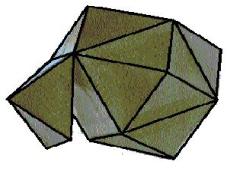
After creating the rhombus dodecahedron in our imagination we now use materialized models for fitting the 6 suitable square pyramids to the sides of a cube using adhesive tape. Then we cut them partially off along the edges with a knife or a razor blade and we get a model enabling us to visualize the fact that the volume of the rhombus dodecahedron is twice the volume of the cube from which it was generated.
Below the phases of transforming the rhombus dodecahedron into two cubes with a common side is illustrated. First, we wind out two pyramids from the opposite sides of the cube, which is located inside the dodecahedron.
|
|
|
|
|
|
Fig. 3 |
|||
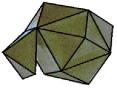
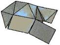
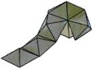
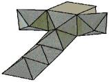
Then we detach the remaining pyramids successively and put them in the line one by one. Finally we fit them together to the second cube.
|
|
|
|
|
|
Fig. 4 |
|||
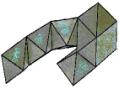
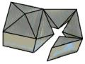
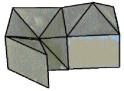
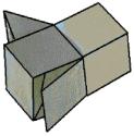
It is easy to recognize that the edge of the rhombus dodecahedron is one half of a spatial diagonal line of the cube. This means that for the edge „a” of the cube, the edge of the rhombus dodecahedron is
![]()
This gives to us an easy derivation of the formula for the volume of the rhombus dodecahedron with the edge b:
 .
.
The reader is able to calculate in the mind the surface of the rhombus dodecahedron with side “b”. The fact that one rhombus dodecahedron with the edge „b” may be transformed into two cubes of the edge „a” allows us to make further deductions. From eight cubes, each of the edge a, we may create another cube with an edge of double length (because 23 = 8). Based on the preceding reasoning, the eight cubes may be transformed into four rhombus dodecahedron. This means that into the cube of the edge “2a” we may pack four rhombus dodecahedrons of the edge
![]()
But how is that? The easiest way would be to reverse the transformation into the cubes and square pyramids. It is, however, not as convenient as it might be supposed. Let’s try something different. First put one such dodecahedron into the cube of the double length edge of the cube, from which it was created, Fig. 5. Recognize that the distance between vertices of the rhombus dodecahedron the opposite situated is the height of that cube. |
|
|
Fig. 5 |
|
|
Fig. 6 suggests how it should be done. We are aware that the dodecahedron dissected into four congruent heptahedrons could be positioned onto the bottom of the cube. One of its edges equals the cube’s edge with the length „2a”. Now it is clear, that to each of the heptahedrons belong: |
|
|
Fig. 6 |
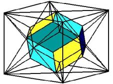
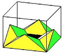
four faces which are isosceles triangles with the base of length
of aÖ2, side of length of aÖ2/2 and the height of a/2,
the rhombus with the length diagonal aÖ2 and a,
two rectangular isosceles triangles with the hypotenuse 2a and the
leg of right angled of length aÖ2.
|
It is interesting that four such heptahedrons create one rhombus dodecahedron - the same one that has been put into the cube. Do you know how many of these heptahedrons you can place in the cube with the edge „2a”? Try to figure it out: the volume of this cube is 8a3, so you can place 8 cubes with the side „a” inside. Each couple of them has the same volume of the one adequate dodecahedron. It means, that inside the cube, which you are just beginning to fill, you can place four rhombus dodecahedrons that are exactly sixteen heptahedrons. |
|
|
Fig. 7 |
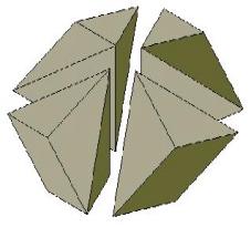
Is it posible?
|
= |
|
? |
|
Fig. 8 |
|||
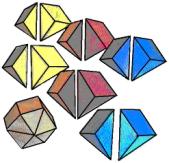
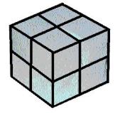
Try to perform it and assemble this cube.
|
|
|
|
|
|
Fig. 9 |
|||
|
At last we show the net of the “magic” heptahedron including its measurement. |
|
|
Fig. 10 |
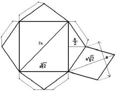
By using Cabri II it is also possible to illustrate the cyclical transformation of all Plato’s polyhedrons. We begin here with cube, across tetrahedron, octahedron, icosahedron, dodecahedron back to cube (see Figures 9 and 10).
|
|
|
|
|
|
|
|
|
|
|
|
|
|
|
|
|
|
|
|
|
|
|
|
|
|
Fig. 11 |
|||
By using Cabri II I can also create the Stella octangulla of Johannes Kepler from the cube:
|
|
|
|
|
|
Fig. 12 |
|||
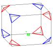
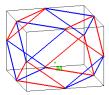
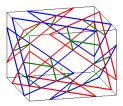
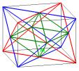
Finally I present the worksheets, which are used in the investigation:
worksheet 1
DRAW THIS POLYHEDRON IN THE WAY YOU SEE IT IN YOUR IMAGINATION.
worksheet 2
ON THIS SHEET, ANSWER THE FOLLOWING QUESTIONS:
|
1 |
The created polyhedron has |
|
vertices. |
||
|
|
|
|
|
||
|
2 |
This polyhedron has |
|
edges. |
||
|
|
|
|
|
||
|
3 |
The faces of this polyhedron are |
|
|||
|
|
|
|
|||
|
4 |
The faces |
ARE/ARE NOT |
congruent. |
||
|
|
|
|
|
||
|
5 |
This polyhedrons has |
|
faces. |
||
|
|
|
HOW MANY? |
|
||
|
6 |
This polyhedron |
IS/IS NOT |
regular |
||
|
|
|
|
|
||
|
7 |
The volume of the polyhedron is |
|
times bigger |
||
|
|
|
HOW MANY? |
|
||
|
|
than the volume of the adequate cube. |
||||
Cubics and quartics on computer
Pavel Pech and Jaroslav Hora
České Budějovice, Plzeň, Czech Republic
In basic courses of geometry at colleges and universities mainly linear and quadratic objects are studied. Using computers enables us to include into these courses also objects, which are described by algebraic equations of higher degree, for example cubics and quartics. Besides standard mathematical software like Maple or Mathematica there has also been a special software developed, by means of which we can demonstrate in a teaching process all the algebraic curves of degree less then five. A catalogue of well-known cubics and quartics is enclosed.
1 Introduction
Linear and quadratic geometry belongs to the main part of a basic course of geometry at colleges and universities. In such a course properties of conics and their higher dimensional analogies are studied. Much time is devoted to the study of basic properties of quadratic forms. Forms of higher degree are rarely studied. One of the reasons could be that solving algebraic equations of degree higher than two is difficult, although there are many geometric objects, which are described by equations of this type.
Problems of higher degree can be tackled more easily, now we have more efficient computers, specialised mathematical software and new theories (Groebner basis of an ideal, elimination theory etc.). More problems in geometry can be addressed by solving equations of higher degrees and by possibly solving of non-linear systems of equations.
We think that basic notions of the theory of algebraic curves and the theory of solving non-linear systems of algebraic equations by means of Groebner basis of ideal should appear at schools. Especially algebraic curves of degree three and four – cubics and quartics.
2 Cubics and quartics
The equation of a cubic can be written in the form
|
|
|
(1) |
where all the coefficients are real numbers with (a, b, c, d) ¹ (0, 0, 0, 0). Newton (1706) was the first who classified cubics. He claimed that every cubic could be expressed in one of four following forms:
|
|
|
(2) |
|
|
|
(3) |
|
|
|
(4) |
|
|
|
(5) |
By considering the behaviour of cubics at infinity Newton arrived at 72 types of cubics and another 6 were added lately. Newton also made the remarkable assertion that all cubic could be obtained from those in (4) by a central projection between two planes. A similar situation occurs in the case of conics, which can be all projected from an arbitrary one and be expressed as a planar section on the cone. This group (4) of cubics is also called elliptic curves, which played an important role in the proof of Fermat’s Last Theorem done by A. Wiles in 1995.
How to draw an arbitrary cubic given by the equation (1)? We adjust (1) in the form
|
|
|
(6) |
where the coefficients A, B, C, D depend on x and solve it with respect to the unknown y. To an arbitrary value x there exist at most three real values y satisfying (6). It is obvious that such a solution can be done only by means of a computer. A program was developed; see J. Fanfrlík (1997), or J. Hudeček (1998), which can draw an arbitrary cubic given by (1). To draw cubics we can also take advantage of a common software (Maple, Mathematica) to put an equation into a parametric form or to use a direct command implicitplot in Maple. Special software based on a solution of systems of algebraic non linear equations enables us to express cubics both in an implicit and a parametric form.
The equation of an arbitrary quartic is as follows
|
|
|||
|
|
where |
|
(7) |
L. Euler divided quartics into eight types; see Euler (1748), or Hudeček (1998). To draw an arbitrary quartic given by the equation (7) we view it in the form
|
|
|
(8) |
where the coefficients A, B, C, D, E depend on x. Solve (8) with respect to the unknown y. For an arbitrary value x there exist at most four values y satisfying (8).
Example 1: We are given a parabola with the parameter p. Find a locus of feet of perpendiculars dropped from the vertex of the parabola all its tangents {pedal curve}.
Solution: Students know that the locus of feet of perpendiculars dropped from the focus of a parabola to all its tangents is its directrix. Our problem is a generalization. Choose the coordinate system so that the parabola has the equation y2 = -2px. At an arbitrary point X = [x1, y1] of the parabola construct the tangent
|
|
|
|
The line l going through the vertex of the parabola, which is perpendicular to t, has the equation
|
|
|
|
Then the point of intersection of the lines t and l has coordinates [x, y], where
|
|
|
|
Eliminating the variables x1, y1 after a short calculation we arrive at
|
|
|
(9) |
which is the equation of Cissoid of Diocles, Fig. 1. We see that (9) is an algebraic equation of the third degree and the curve is a cubic.
|
|
|
|
|
Fig. 1: Parabola with its pedal curve – Cissoid of Diocles |
||
Now we shall execute the last part part of this example with Mathematica. We put
Eliminate[{y*y[1]==-p*(x+x[1]),y==y[1]/p*x,y[1]^2==-2p*x[1]},
{x[1],y[1]}]
and immediately get
|
|
|
|
which is the same as (9). In Fig. 1 there is a parabola with the parameter p=2 with its pedal curve – cissoid of Diocles drawn in Maple obtained by
a:plots[implicitplot](x^3+x*y^2-y^2,x=-3..3,y=3..3,scaling=constrained,grid[200,200]:
b:plots[implicitplot](y^2+4*x=0,x=-3..3,y=-3..3, scaling=constrained,grid[200,200]:
display({a,b});
Example 2: Determine the locus of points X in a plane whose product of distances to two given points F1, F2 is constant.
Solution: Students know the locus of points, whose sum (or difference) of distances to two given points is constant. It is quite natural to ask, what will arise if we replace the words „sum“ or „difference“ by the word „product“. Choose Cartesian coordinate system so that F1 = [-e, 0] F2 = [e, 0] . Denote the value of the product of distances of the point X = [x, y] to the points F1, F2 by a2 . We determine the set
|
|
|
(10) |
Expressing (10) in the form
|
|
|
|
we get
|
|
|
(11) |
|
|
|
|
|
|
Fig. 2: Lemniscate of Bernoulli |
|
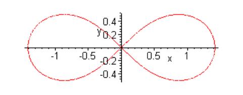
We see that (11) is an algebraic equation of the fourth degree and the curve k satisfying it, is a quartic – Cassinian oval Shikin (1995). If we put a = e we get the well-known Lemiscate of Bernoulli, Fig.2. To obtain Fig. 2 we entered in Maple
plots[implicitplot](x^4+2*x^2*y^2+y^4-2*x^2+2*y^2=0,x=3..3,y=3
..3,scaling=constrained,grid[200,200];
Example 3: Write the implicit equation of the curve, which is given by parametric equations
|
|
|
|
Solution: We put in Maple
Eliminate[{x=(3*a*t)/(t^3+1),y=(3*a*t^2)/(t^3+1)},t];
and obtain
|
|
|
|
The second relation means, that the implicit equation of the curve given above is
|
|
|
|
which is the well-known cubic Folium of Descartes. To draw this figure we could either use the previous way
plots[implicitplot](x^3+y^3-5*x*y=0,x=-3..3,y=3..3,scaling=con constrained,grid[200,200]);
or we could type
with(plots):
a:=plot([(3*a*t)/(t^3+1),(3*a*t^2)/(t^3+1),t=-infinity..-1]):
b:=plot([(3*a*t)/(t^3+1),(3*a*t^2)/(t^3+1),t=-1..infinity]):
display([{a,b}])
and obtain Fig.3 for suitable value a.
|
|
|
|
|
|
Fig.3 |
|
3 Conclusion
The text above gives a brief overview of using computer by investigating cubics and quartics. To know the software, which was developed at the University of South Bohemia including the catalogue of cubics and quartics, contact please one of the authors.
Acknowledgement: I am pleased to acknowledge my indebtedness to Professor Jean Flower for thorough reading the text, her comments and improving the language.
References
Bix, R. (1998) Conics and cubics: a concrete introduction to algebraic curves. Springer.
Euler, L. (1748) Introductio in analysin infinitorum. Tomus II., Lausanne.
Fanfrlík, J. (1997) Křivky třetího stupně a jejich klasifikace. Diploma thesis, Univ. South Bohemia, České Budějovice.
Hudeček, J. (1998) Křivky čtvrtého stupně. Diploma thesis, Univ. South Bohemia, České Budějovice.
Newton, I. (1706) Enumeratio linearum tertii ordinis. London.
Shikin, E. V. (1995) Handbook and Atlas of Curves. CRC Press, Boca Raton.
Expression equivalence checking
in Computer Algebra Systems
Eno Tõnisson
Tartu, Estonia
2. Mathematics syllabus and CAS. What needs to be changed?
3. Educational applications of expression equivalence checking
4. Test compilation principles
7. Equation equivalence and answer checking
This paper investigates the possible educational application of equivalence checking and the capability of expression equivalence checking in some common computer algebra systems. The applications of equivalence checking can be analysed from the viewpoint of three types of users: that of the teacher, that of the student, and that of an Intelligent Tutoring System. This paper deals with the way a computer algebra system copes with the checking of the basic equivalences of algebra and trigonometry. It appears that the tools are far from perfect and require improvements.
1 Introduction
Computers have been introduced in schools in large numbers already; many schools also possess computer algebra systems. A large number of enthusiastic school and university teachers have invented hundreds of sophisticated methods for doing reasonable work with the existing computer algebra systems. However, the use of these requires additional efforts and presupposes a better understanding of computer algebra systems and mathematics than we can expect from an average teacher.
How can we more effectively apply computer algebra systems in mathematics learning and teaching? Roughly speaking, their effectiveness depends on the mathematics syllabus and standards on the one hand and the computer algebra systems on the other. Either of them is subject to change in the course of time, and we need to find out what we should keep in mind as we implement these changes. Some aspects of this question are addressed in Section 3. The changes will certainly lead to modifications in the list, depth and style of the syllabus topics. Whatever the exact nature of the changes, it seems that effective equivalence checking devices will have a very important and increasingly influential place in the process. The possible educational applications of equivalence checking are described in more detail in Section 4.
Different computer algebra systems provide slightly different tools for checking the equivalence of expressions. There are special commands (for instance, testeq in Maple) that use probabilistic trial algorithms. The focus, however, has been laid on the means of simplifying the difference between expressions. Simplification belongs to the basic features of any computer algebra system. A more detailed analysis of the example selection criteria is given in Section 5.
The bulk of this paper is constituted by the results of experiments presented in Sections 6 and 7. The general scheme is similar to the review (Tõnisson 2000) edited by Michael J. Wester, which introduces the resources of computer algebra systems for solving various problems. However, the issue of equivalence is not addressed directly there. The examples in this article deal with the basic equivalences of algebra and trigonometry, which can be found in many textbooks, manuals and reference books. In addition, some school problems have been analysed. These topics have been selected because they are good examples of expression manipulation. Expression manipulation, morever, plays a prominent part both at a school and a university level, in one form or another. The expressions that pose no problems in an equivalence checking have been listed above the tables. The examples that are more interesting have been placed into tables.
The following versions of computer algebra systems were used in the experiments:
DERIVE for Windows. Version 4.11 (1996)
Maple V Release 5. Student Version 5.00 (1998)
Mathematica for Students. Version 3.0 (1996)
MuPAD Version 2.0 (2001)
At the end of this paper, some concluding remarks are given.
2 Mathematics syllabus and CAS. What needs to be changed?
It is clear that part of school mathematics is too complex, impractical or even virtually impossible to teach and learn using computer algebra systems. On the other hand, it is equally clear that a great deal of topics, approaches and problem types that could be handled using computer algebra systems are disregarded at school, at least at present. How, then, can we apply computer algebra systems in a more effective way?
We can imagine several different developments for the future. One possible approach is to critically review the mathematics syllabus and standards and make relatively fundamental changes there, which would result in computer algebra systems being more applicable to school. For instance, it is possible to reduce the number of indispensable manual calculation skills. This might be done at several levels, for instance, not requiring the student to solve a quadratic equation without a calculator any longer (see Herget e.a. 2000). In changing school mathematics standards, consideration must be given to the training and readiness of teachers. The 31 teachers that participated in a year-long training cycle “Computers in School Mathematics” were asked the following question: “To what extent should the mathematics syllabus be changed in light of the possibilities of information technology?” All of them believed that changes in the syllabus are necessary. Approximately 2/3 of the respondents were in favor of small changes, 1/3 of greater changes, and one respondent of fundamental changes. When the respondents were asked to imagine a situation in which all teachers would possess computer skills at least equal to those of their own, 2/3 of the respondents stood for greater changes, 1/3 for small changes and two for fundamental changes (see Tõnisson 2000). Of course, a small questionnaire like this provides no good statistical grounds for generalizations; however, it may still be maintained that teachers show readiness for moderate changes, and that a rise in the level of their computer skills will only increase that.
The other answer is to maintain the existing approaches (topics, presentation styles, etc.) in the syllabus and try to use or modify the existing computer algebra systems for their implementation. Here the level of mathematical systems plays an important role. To what extent do they already possess the features required for learning purposes? Can we hope that such perfect systems will emerge in the immediate future? Why are intelligent systems that might render mathematics teaching more effective still uncommon?
What, then, are the weaknesses of the existing computer algebra systems? One of them is apparently the imperfections of the step-by-step solution feature. As a rule, computer algebra systems solve problems in one step, as a “black box”. In the simplest form of use, the system is simply given the task of solving a problem or making a step using the solution algorithm. Such a method, however, provides the student with few opportunities to gain new knowledge, and none for making mistakes.
Many teachers seem to reject the use of computer algebra systems by a very simple reason: they are afraid of "the calculator effect", amplified by the far greater capacity of the increasingly powerful computer algebra systems of today. Many teachers would be interested in computerizing math problems in a more conservative way, where the steps are made by the student himself whereas the program verifies the accuracy and reasonability of the results. Whatever the exact trend of development, we need to clarify what fields are particularly important for effective application of computer algebra systems. One of them is undoubtedly expression equivalence. Besides, it may be maintained that equivalence checking is a prerequisite to precluding the “calculator effect”. This, however, is not the only important characteristic of equivalence checking. In the next section, we will analyze some of the applications of equivalence checking.
3 Educational applications of expression equivalence checking
In the process of teaching mathematics, the applications of equivalence checking can be analyzed from the viewpoint of three types of users: that of the teacher, that of the student, and that of the Intelligent Tutoring System.
It is possible to effectively use computer algebra systems in case the command for equivalence checking is given by the student. If, in doing a transformation problem (or in solving equations and equation systems), the student gets a different answer than that given in the textbook, does it necessarily mean that he has made a mistake? A computer algebra system provides an easy means of equivalence checking. (See Kutzler 1996). It also allows checking one’s work at each step. In an expression manipulation problem the student will enter the next line and then check whether it is equivalent to the previous one. If it is not, he will find the error and then enter the next line. This does not restrict the student’s right to make mistakes while it facilitates the spotting of them. Compared to writing on paper it is now easier to create new and often long lines by copying. This reduces the risk of transcription errors. Apart from the ordinary application, where the user is able to check whether a manipulation line is equivalent to the previous one, it is possible to apply new didactic approaches, in which the automatic checking of expression equivalence is more and more integrated into the learning process.
One important reason for considering expression equivalence is the fact that in solving their problems, students often perform transformations in a relatively routine way, not necessarily understanding whether and why they can be done, whether equivalence has been secured, etc. The fact that computer algebra systems enable the student to divide his attention in a different way in performing transformations should lead to a rise in the importance of expression equivalence.
Of course, a number of questions arise: What changes should we make in the problems? For what purpose? What do we need to check? What should be the structure of math examinations? These are all interesting questions; however, they will not be given detailed treatment in this paper.
Expression equivalence checking resources that are functioning properly in computer algebra systems would also provide better opportunities for teachers, who would be able to easily check their students’ voluminous manipulation exercises. For instance, errors in a manipulation problem may be spotted by first checking the equivalence between the beginning and the end of the manipulation and then determine the exact location of the error by applying the concept of binary search.
A promising area is using computer algebra systems in the Domain Expert Module of an Intelligent Tutoring System which capable of giving adequate feedback and hints. If, in the process of problem solving, the student enters an expression, it is necessary to check its syntax, its equivalence to the previous expression, the compliance of the manipulation direction with the algorithm, and the completeness of the algorithm step. The Domain Expert Module might be able to provide the resources for an intelligent tutoring system. The existence of a mechanism for checking the equivalence of expressions is extremely important in the creation of such an intelligent tutoring system. One such system, Math Assistant, which has been designed for teaching an introductory course of mathematical logic for first-year students of mathematics, has been described in articles (Prank 1991, Prank and Viira 2001). However, equivalence checking is very simple when it comes to propositional logic. It does not require a sophisticated domain expert. In algebra and some other fields of mathematics the main component of the Domain Expert of the respective intelligent tutoring system may be constituted by a computer algebra system (Prank and Tõnisson 2001).
4 Test compilation principles
The above would make sense if computer algebra systems were able to perform equivalence checking. Are they, however?
Computer algebra systems are capable of solving a large number of fairly voluminous problems. In several instances, however, the analysis of the more problematic special cases is largely ignored. This is left for the user himself to handle. To be usable in an educational setting, the system should confine itself to dealing with less voluminous examples while being able to correctly solve all problematic cases. A large share of the examples presented in this article are elementary equivalences, which the student should know and master. Similar sets of examples can be found in a number of writings, and virtually all of them have been included in educational syllabuses in all the countries of the world. (The extent to which they are practically required depends, of course, on a particular syllabus. It may vary on both the international and the domestic scale.) Apart from these, some problems from school textbooks as well as exercise sets have been presented to test the identification of equivalence in expressions that are slightly more complicated. At any rate, the problems are simple in mathematical terms. Special treatment is given to the so-called “insidious example”
|
|
|
|
in which “bugs” can be expected.
Of the computer algebra systems under study, only Maple has a command for checking the equivalence of expressions, testeq. The command checks the equivalence probabilistically. It can identify almost all the equivalences under study, as well as the equations presented for proof in textbooks. Only in the case of a few expressions does it issue the Fail message. Such a probabilistic approach is undoubtedly fruitful; however, it is not suitable for every situation. The test commands in Mathematica, SameQ and Equal, issue a True message only if the expressions are absolutely identical. Here automatic simplification plays a prominent part, transforming the sides of the following equivalences into an identical form. For instance, a/1 will automatically be transformed into a. In the following section, such equivalences have been marked with (I).
The bulk of the tests consists of the analysis of whether the difference between the supposedly equivalent expressions is reduced to zero after running the command Simplify. (There are no assumptions for the operands.) An added effect is demonstrated after processing the expressions previously by the command Expand. The tables includes the abbreviations S (instead of simplify(expr1-expr2) ) and S+E (instead of simplify(expand(expr1)-expand(expr2)) ), which enable subsequent tables to be composed in a more space–saving manner. Computer algebra systems also include other, more specific simplification commands. Although they may improve the results, they have not been used for the sake of simplicity. Mark 0 in the tables indicates that the result of simplification is 0, mark No indicates the result of simplification is not 0.
There are different reasons why computer algebra systems cannot always cope with equivalence checking. They include mathematical reasons (this kind of problems are not always solvable), or other reasons; however, in some cases, it seems that the authors of computer algebra systems have simply paid too little attention to this topic. The reasons have not been analyzed in this paper.
5 Algebraic equivalences
All the computer algebra systems under study claim the following equivalences to be valid (testeq in Maple will issue a true message and all attempts at difference simplification will give a zero.):
(I) indicates equivalences the sides of which are automatically transformed into an identical form in Mathematica:
|
|
|
|
|
|
|
|
|
|
|
|
|
|
|
|
|
|
|
|
|
|
|
|
|
(O) indicates equivalences in which in MuPAD simplify(expr1-expr2) does not result in zero but simplify(expr2-expr1) does:
|
|
|
|
|
|
|
|
|
|
|
|
Without any problems, a0 and 1 are also considered equivalent, which, however, is not the case with all numbers. (For instance, if a = 0). Such special cases (e. g. division by zero, logarithm restrictions) may be pointed out here and hereafter, but they are not dealt with in this paper.
Table 1: Algebraic equivalences
|
Equivalence |
Maple testeq |
Maple S, S+E |
M-matica S, S+E |
Derive S, S+E |
MuPAD S, S+E |
|
|
true |
0, 0 |
0, 0 |
0, 0 |
No, No |
|
|
true |
0, 0 |
0, 0 |
0, 0 |
0,No(O) |
|
|
true |
No,No |
No,No |
No,No |
0, 0 (O) |
|
|
true |
No,No |
No,No |
No,No |
0,No(O) |
|
|
FAIL |
No,No |
No,No |
0, 0 |
0,No(O) |
|
|
true |
0, 0 |
0, 0 |
0, 0 |
No, No |
|
|
FAIL |
0, 0 |
No,No |
0, 0 |
No, No |
|
|
true |
No,No |
No,No |
No,No |
No, No |
|
|
true |
0, 0 |
0, 0 |
0, 0 |
No, 0 |
|
|
FAIL |
No,No |
No,No |
No,No |
No, No |
|
|
FAIL |
0, 0 |
0, 0 |
0, 0 |
No, No |
|
|
FAIL |
No,No |
No,No |
No,No |
Error |
Table 2: “Insidious” Problem
|
Equivalence |
Maple Testeq |
Maple S, S+E |
M-matica S, S+E |
Derive S, S+E |
MuPAD S, S+E |
|
|
true |
0, 0 |
0, 0 |
0, 0 |
0, 0 |
Some examples of textbook problems are presented at www.ut.ee/~eno/equivalence/.
6 Trigonometric equivalences
All the computer algebra systems under study claim the following equivalences to be valid:
|
|
|
|
|
|
|
|
|
|
Table 3: Trigonometric equivalences
|
Equivalence |
Maple testeq |
Maple S, S+E |
M-matica S, S+E |
Derive S, S+E |
MuPADS, S+E |
|
|
true |
0, 0 |
0, 0 |
0, 0 |
No, 0 |
|
(+ 3 others) |
true |
No, 0 |
0, 0 |
No, No |
0, 0 |
|
|
true |
No, 0 |
0, 0 |
No, No |
No, 0 |
|
|
true |
No, 0 |
0, 0 |
No, No |
No, 0 |
|
|
true |
0, 0 |
0, 0 |
No, No |
No, 0 |
|
(+3others) |
true |
No, 0 |
0, 0 |
No, No |
0, 0 |
|
(+ 3 others) |
true |
No, No |
0, 0 |
0, 0 |
0, 0 |
|
|
true |
0, 0 |
0, 0 |
0, 0 |
No, 0 |
Textbook examples are presented at www.ut.ee/~eno/equivalence/ . Here, we might point out the problem
![]()
the equivalence of which could not be established with the help of command lines by any of the systems under study.
7 Equation equivalence and answer checking
The issue of checking the equivalence between expressions is closely connected with that of the equivalence between equations (and also equation systems). Checking of the equivalence (= equality of the sets of solutions) of equations and systems of equations is not implemented in computer algebra systems. They also do not check correctness of the solutions found by themselves and they can output extraneous solutions already in quite simple situations. For example (Mathematica):
In[1]:= Solve[x(x-1)/(x-1)==1]
Out[1] = {{x->1}}.
It is taught at school that answers need to be checked. If the student uses a computer algebra system to check the correctness of a solution, then in many cases the computer algebra system simplifies the equation before substituting the values of the variables and repeats the mistake made during the solution process:
In[3]:=ReplaceAll[x(x-1)/(x-1)==1,x->1]
Out[4] = True.
8 Conclusions
The tables largely speak for themselves. Clearly, the existing computer algebra systems cannot be completely relied on in checking the equivalence of expressions. Furthermore, one cannot recommend a particular possibility to the student, for instance – even the command testeq does not function perfectly. This, however, will undoubtedly reduce the possibilities of using computer algebra systems in an educational setting, since both the student and the teacher need a device that can be relied upon in equivalence checking. Furthermore, the existing devices are not fully fit for creating an intelligent system. Hopefully, the developers of computer algebra systems will find a way for improving the resources that are still inadequate to be applied for educational purposes. By this, we give an opportunity to more effectively apply computer algebra systems.
Acknowledgement. The Estonian Science Foundation supports the writing of my doctoral thesis.
References
Herget, W., Heugl, H., Kutzler, B., Lehmann, E. (2000) Indispensable Manual Calculation Skills in a CAS Environment. http://www.kutzler.com/
Kutzler, B. (1996) Improving Mathematics Teaching with DERIVE. Chatwell-Bratt.
Prank, R. (1991) Using Computerised Exercises on Mathematical Logic. Informatik-Fachberichte. 292. Springer, 34-38.
Prank, R., Tonisson, E. (2001) Is the Domain Expert Module for expression manipulation exercises ready? Proc. of the Tenth Intern. PEG Conference 2001, 51-56.
Prank, R., Viira, H. (1991) Algebraic Manipulation Assistant for Propositional Logic. Computerised Logic Teaching Bulletin. St Andrews Univ. 4, 13-18.
Tõnisson, E. (2000) Matemaatika ainekava infotehnoloogia võimalustest lähtuvalt. Konverentsi Reaalained ja uus õppekava materjalid. Tartu 2000, 166-175.
Wester, M. J. (ed.) (1999) Computer algebra systems: a practical guide. J. Wiley, New York.
[1] A global control criterion is used to check the correctness of the whole exercise (e.g. the verification of the equations solutions). A local control criterion is used to check a limited part of the treatment of the exercise (e.g. checking an arithmetic operation or an application of the distributive property used during the solution of an equation).
[2] B Gymnasiou: second class of junior high school (8th year of compulsory education)
[3] By interviewing 25 junior-high school teachers we have found that the average time that they devote on self-correction activities is 1,5 hours concerning 1st degree equations. The self-correction activities that they realise are based on traditional arithmetic verification. So, the self-correction activities realised in comparison classes can be considered as an extended and more systematic work of the same type as the self-correction work which is often done in ordinary teaching of the subject.