Strand 1:
Integration of IC technologies
into learning processes
Jean-Baptiste Lagrange
Rennes, France
|
Plenary lecture |
Computer-rich learning environments and the construction of abstract algebraic concepts |
|
Differentiating mathematics instruction through technology: Deliberations about mapping personalized learning |
|
|
Mathematical software in the educational process of the French and Hungarian teachers |
|
|
Observing student working styles when using graphic calculators |
|
|
Diagnosing mathematical needs and following them up |
|
|
The impact of training for students on their learning of mathematics with a graphical calculator |
|
|
Data collection and manipulation using graphic calculators with 10-14 year olds |
|
|
The role of the graphic calculator in early algebra lessons |
|
|
The ODE curriculum: Traditional vs. non-traditional. The case of one student |
|
|
Experimental mathematics |
|
|
Cognitive and didactic ideas designed in TIC environments for the learning and teaching of arithmetic and pre-algebra knowledge and concepts |
|
|
To learn from and make history of maths with the help of ICT |
|
|
Thinking the unthinkable —Understanding 4 dimensions |
|
|
Remedial education of quadratic functions using a web-based on-line exercise system |
|
|
Integrating mathematics, physics and Interactive Digital Video |
|
|
How to use computer-based learning effectively in mathematics |
|
|
The visualisation of parameters |
|
|
Functional algebra with the use of the graphing calculator |
International conferences on technology in mathematics teaching offer great opportunities to consider new developments of technology and powerful ideas for their introduction into teaching and learning. ICTMT 5 really opened new visions for the use of innovative technological environments with great potential for challenging students to investigate richer problems.
Like other strands and working groups, these new prospects were the centre of Strand One's presentations and discussions. The specific reflection in the strand was that, to achieve the integration of IC Technologies into learning processes, new visions and powerful ideas are not by themselves sufficient. The challenge IC technologies in Education have to meet, is to understand better the students' functioning and learning processes when using technology, and the new teaching contexts
The plenary talk by Dreyfus was an authoritative introduction. Addressing the case of the construction of abstract algebraic concepts, he emphasised the help that the computer can provide to support innovative alternative approaches using the large variety of multi-representational tools now available. He also stressed the need for an urgent reflection drawing on examples of success as well as failure in using technology for students' construction of meaning. Looking at possible reasons for failure, he focused on the potential ambiguity of representatives for mathematical objects in technological representations. He also showed the importance and difficulties of an appropriate design of the students’ task: learning situations with technology are very new and foreseeing students' procedures and conceptualisations is never obvious.
He made the point that we have to deepen our understanding of students’ functioning and learning processes and he outlined a new cognitive framework related to abstraction that issued of research on the use of technology. His paper in these proceedings provides an outline of the associated research program.
Contributions
The plenary was followed by seventeen contributing talks. There is no simple approach to the complexity of learning processes especially when using technology and it is therefore not surprising that contributions cannot be easily classified into subgroups addressing the same issue. I will nevertheless try to introduce a classification with regards to what I see as the main trend in each contribution.
In three contributions, the main trend could be the change that technology potentially brings into the mathematical registers of expression and activity. Chrisden’s point was that technology changes the nature of the mathematical activity. As experimenting has a growing impact on professional mathematicians, it should also become part of our teaching strategies. Habre's approach was that technology brings new powerful means for investigating a topic like differential equations. The computer helps to display a graphic showing a family of solutions and then the students will be able to concentrate on a geometrical study of solutions, possibly more meaningful than the usual symbolic computation of solutions. Forrester stressed also that computer representations would provide new means to investigate and understand mathematical phenomena. Young students with no formal teaching in statistics were able to use and interpret the output of Graphic Calculators when manipulating data that were familiar to them.
Four other contributions were centred on a new task or a set of tasks that appear to be relevant when using technology. Gage showed how the evaluation of expressions with variables by a calculator could be a basis for tasks to favour the students' construction of a conception of algebraic variables. Pappas introduced us to Digital Video Technologies and how it can be used as a connecting link between mathematics and science, helping students understand the role of a co-ordinate system. van de Giessen presented a piece of software as means to dynamically investigate graphs. The notion of 'sliding parameter' is associated with a changing graph and the student is able to make the next step towards a family of parameters. van der Kooij showed how manipulating graphs on a calculator can be the basis for new approaches to functional thinking, especially for students non receptive to a traditional symbolic approach to algebra.
In four further contributions, the new teaching and learning situations were the point of interest. Situations were autonomous learning using a Computer-Based Learning environment (Pitcher), remedial work by way of a Web-based On-line Exercise System (Nishizawa), the use of the wealth of means that IC technologies offers to explore mathematical ideas and to communicate (Loeman) or a system for mathematical diagnosis and follow up (Challis) helping a university to better meet what society is today requiring from upper secondary teaching. In the latter case, the global teaching and learning situation in a mathematical department is affected by the use of new technology. In these four contributions, the particular demands that technologies imply for students' work are discussed in relation with their learning processes.
Two contributors focused especially on the teachers. Alagic reported from her experience of a graduate course for teachers aiming to use the power of IC technologies to differentiate mathematics instruction. She showed what theoretical reflection we need if we want to really help teachers to adequately use the technological tools. Bako questioned university teachers and students on what they knew about software that could be used to teach and learn Mathematics and about their view on this use. Answers are sometimes disconcerting because they show surprising gaps and misunderstanding between university and secondary schools about the educational use of technology.
Three contributions appear to me as especially interested in the psychological or ‘cognitive’ aspects of learning with technology. Meyer-Bothling reminded us of what is known of human perception and its faculty of adaptation. From this, he developed a stimulating project of training to allow people to enter into the fourth dimension. Smith’s interest was in the observation of student’s procedures when doing tasks on a calculator. He presented a special piece of software to help teachers or researchers to do this observation. Lemoyne developed some cognitive ideas for the learning and teaching of arithmetic and pre-algebra knowledge, and showed how these ideas can be implemented in the design of computer learning environments.
Finally, there is one more issue: students develop varied representations of a technological tool depending on how they learned to use it, and these representations have a great impact on how they learn mathematics with this tool. In my opinion, Fentem addressed especially this question and offered a research methodology for its study. His contribution has interesting connections with the idea of ‘instrumentation’ that a number of researchers are now considering (see for instance Lagrange, 1999; Trouche, 2000).
The above classification is based on ideas that can be seen as the bigger trends in the contributions, but each contributor addressed several of these and the discussion raised even more questions. So, beyond this tentative classification, the seventeen contributions and the plenary address are a web of interwoven concerns. The Strand illustrated well the idea that the complexity of teaching and learning with technology cannot be understood with a uni-dimensional approach and really gave matter for reflection on what could be a multi-dimensional approach. This is a great satisfaction for the chair of this Strand who is working in a research team aiming at a 'multidimensional framework' to tackle the integration of IC Technologies (see Lagrange, Artigue, Laborde, Trouche, 2001).
References
Lagrange, J.B. (1999) Complex calculators in the classroom: theoretical and practical reflections on teaching pre-calculus. International Journal of Computers for Mathematical Learning, 4.1, 51-81.
Lagrange, J.B., Artigue, M., Laborde, C., Trouche, L. (2001) A meta study on IC Technologies in Education. Towards a multidimensional framework to tackle their integration into the teaching of mathematics. In M. van den Heuvel-Panhuizen (ed.) Proceedings of PME 25, University of Utrecht, July 2001 Vol 1, 111-122.
Trouche L. (2000) La parabole du gaucher et de la casserole à bec verseur: étude des processus d'apprentissage dans un environnement de calculatrices complexes. Educational Studies in Mathematics 41, 239-264.
Computer-rich learning environments and
the construction of abstract algebraic concepts
Tommy Dreyfus
Tel Aviv, Israel
1. Linear algebra: A principled technology-based approach
There are many beautiful mathematical demonstrations with computers and many attractive educational software programs. On first sight, many of them appear useful to me, and probably to most of you. They are impressive to mathematicians and educators. But do they achieve the aims of designers and teachers? And do we know why they do or do not achieve these aims?
In many cases we don't. Research results are inconsistent at best (Blanton, Moorman and Trathen, 1998; Fabos and Young, 1999). One reason for this is that technology is usually a very small part of the learning environment. Mathematics curriculum development for computerized environments is a complex activity involving continuous and long-term interaction between designers, researchers, teachers and learners (Hershkowitz, Dreyfus, Ben-Zvi, Friedlander, Hadas, Resnick and Tabach, in press). It typically includes trials with small groups (often successful); first classroom trials (often after considerable revision) and large-scale implementation which has its very own problems; often these are connected to the conservatism of the educational systems and teachers' difficulties to change their ways of thinking and classroom behaviour.
But even on the smallest scale and even with the most careful theory-based preparation, success is far from assured. There are failures that often go unreported, and we should look at them and learn from them. More specifically, even a careful, principled didactic design may be of limited help in supporting students’ development of abstract mathematical notions. The aim of this paper is to illustrate this claim and to suggest that research on processes of abstraction in context might provide helpful insights.
Indeed, as compared to the amount of software development and teaching proposals, among others at conferences like ICTMT, there is a dearth of well-founded research-based knowledge about learning with computers. In a recent survey of over 600 publications on ICT in mathematics education, Lagrange, Artigue, Laborde and Trouche (2001) have made the following observation: Even though their selection was somewhat biased because of their own preoccupation with research and because they are based in a country with a strong research tradition, they have found that in the recent literature, the vast majority (73%) of publications relate to development rather than research. And more significantly, even among this majority, most papers concentrate on describing the possibilities of the software rather than innovative classroom activities. In other words, we mathematicians and developers excel at sitting at our computers and implementing ingenious ideas for how to put mathematics on the screen. We are less eager to think in depth about classroom activities that could be based on our wonderful ideas and to actually try out these activities in real classrooms. And only a few of us have the means, the background, the time and the inclination to seriously study what happens in terms of teaching and learning when these wonderful software products are being taken to class.
In this paper, I will build on such research on classroom trials. I will sound a cautionary note, using examples of what can go wrong. I will intentionally and consciously chose a biased selection of observations. It is biased toward the less successful experiences, toward the pitfalls, toward the obstacles. I do not refer to logistic problems but to problems with teaching and learning that have been observed to occur in spite of wonderful ideas, in spite of deep thinking on the part of the developers, in spite of careful implementation, and in spite of talented and experienced teachers. I will thus focus on students rather than on software, on learning rather than on teaching, and more specifically on research about the emergence of abstract knowledge structures. I have two reasons for choosing such a bias: One is that researchers understandably prefer to publish their successes rather than their failures. I hope to redress the balance a little bit. The other reason is that I want to make a point, namely the point that it is well worth our while, as a community, to invest considerable resources into the investigation of teaching and learning activities with technological tools: The fact that a piece of software or an ICT activity looks beautiful, convincing and thrilling to us does not mean that it will be either exciting or beneficial to the students for whom it is intended.
Disclaimer: I am not an adversary of the use of technological tools in the classroom – quite the contrary, I believe they can be very useful, I enjoy using them, I do use them when I teach, and I have participated in the development of software and technology-rich teaching activities. But at the same time, I am aware that the effects of my efforts may be different from what I as a developer and teacher expect and predict.
1 Linear algebra: A principled technology-based approach
The teaching and learning of algebra, whether elementary, linear or modern algebra, is an area where computer support might be expected to be particularly useful, for several reasons: A large variety of multi-representational tools are available, the onerous and tedious calculations can easily be taken over by the computer, and most importantly, it has been suggested that appropriate software can be used to bridge the existing gap between the concrete and the abstract (e. g., Schwarz and Dreyfus, 1995).
I will concentrate in the sequel on the teaching and learning of linear algebra, mainly because of my personal experience with teaching, development and research. In linear algebra, just as in other high school and college algebra courses, many suggestions have been made how to use computer tools to enhance the courses. Many of these tools support students’ algebraic and numerical calculations and thus allow them to progress faster and further to realistic applications of linear algebra than would otherwise be possible (e.g., Leon, Herman and Faulkenberry, 1996). In these cases, the software is used mainly as a tool to do mathematics rather than as a didactic aid.
Other software tools are meant to use geometric illustration as a source for the development of intuitions related to linear algebra concepts. The notions of linear transformation and eigenvector/eigenvalue have received special attention in this respect (e.g., Martin, 1997). The computer constructions and visualizations of linear transformations and eigenvectors are sometimes quite ingenious, leading to interesting mathematical problems. They are certainly a joy for the mathematician, but it is not clear if and how they can be useful in the teaching and learning of linear algebra at the undergraduate level. While the mathematics underlying the computer visualizations and descriptions of some technicalities of the design of these visualizations have been studied, few accounts of teaching with their use and of students’ reactions to such teaching are available. It remains unclear whether and to what extent these tools contribute to students’ learning in general and to their construction of abstract linear algebra concepts in particular.
As every college teacher knows, linear algebra is a particularly problematic course because of the high level of abstraction it requires from the students. In a manner quite similar to what happens in high school algebra, students tend to avoid this high level of abstraction by performing actions on a purely formal level. This issue is well documented, for example in Dorier (1997/2000). As a consequence, even the most basic notions of linear algebra, including the very essence of linearity are often poorly mastered and understood by the students. For example, in a recent first year university linear algebra course that was described by the lecturer as conceptually oriented, students were given a transformation from the space P2 of second degree polynomials to the space R2 of real number pairs. The transformation was given by specifying the image of a general second-degree polynomial. Specifically, it was given that the image of the polynomial p or p(x) is the R2 vector T(p) = [p(1), p'(0)], (where p' is the derivative of p). Students were asked to show that the transformation is linear. Somewhat less than half of the students attempted the proof by applying the linearity condition T(k1p1+ k2p2) = k1T(p1) + k2T(p2). Some succeeded with the algebra while others did not. Whether or not they succeeded, their solution provides only limited insight into their understanding of linearity. More interesting is the larger group of students who remembered that the linearity of a transformation is linked to its matrix representation. Most of these students constructed the 2 by 3 matrix

by finding the images of the three basis vectors p1 or p1(x)=1, p2 or p2(x)=x, and p3 or p3(x)=x2 and writing down the matrix whose column vectors are the images T(p1), T(p2) and T(p3). From this they concluded that T is linear since any transformation given by a matrix is linear. They did not realize that in drawing this conclusion they assumed that the transformation is linear. Some students even proceeded to show by explicit calculation that multiplication by the matrix M is a linear operation! The general impression that obtains is that students, even those in conceptually oriented first year liner algebra courses attain only a limited understanding of the central notion of the course: linearity, in particular linearity of a transformation.
More examples of a similar kind have been reported elsewhere (Dreyfus 1997; Dreyfus 1999). Moreover, Hillel and Sierpinska (1994) have reported and further analysed (Hillel, 2000; Sierpinska, 2000) a particularly persistent problem, namely students’ confusion between a vector in Rn and its coordinates in a given basis. These examples show that students tend to avoid reasoning with abstract structures and instead find something to compute. This tendency is facilitated by the arithmetic, Rn based approach to linear algebra, which provides students with vectors and matrices, often numerical ones that entice them to carry out computations without necessarily being aware of their significance.
In a recent project, Sierpinska, Dreyfus and Hillel (1999) have taken a different approach based on an epistemological analysis of entry-level linear algebra. They began from the realization that even in conceptually oriented, Rn based linear algebra courses; computation appears as the all-important issue. They asked themselves whether it is possible to avoid this role for computation by working directly with the concepts. In other words, they aimed to provide students with thinking tools that would allow them to act on vectors without using coordinates and to operate with transformations without using matrices. They also searched for a student centred, constructive manner to do this.
In view of well-known difficulties with the arithmetic Rn approach, they investigated the option of using a geometric entry into linear algebra in two dimensions. They chose to anchor the general notions of vector, transformation, linear transformation and eigenvector in geometric intuitions, by designing a suitable learning environment with the Cabri-geometry II software (Laborde and Bellemain, 1994). The software was used as a didactic tool, not as a tool for solving problems in linear algebra. Its role was to provide a solid conceptual basis for the notions of vector, transformation, linear transformation and eigenvector. The approach was thus conceptual rather than technical. Vectors were represented by arrows pointing from a fixed origin to a general point in the plane. Neither coordinate axes nor coordinates were presented or used at this stage. Operations on vectors (addition, multiplication by a scalar, linear combination) as well as transformations (not necessarily linear) were introduced geometrically. Transformations were represented in by a pair of vectors, a vector v that could be dragged freely to represent the vector to be transformed, and a dependent vector T(v), its image. Dragging v caused T(v) to move according to the rules of the transformation. Linearity of a transformation was introduced, first intuitively and then formally, as compatibility of the transformation with the operations on vectors. The notion of transformation naturally led to the question of the relation between a vector and its image, for example, whether the images of two (or more) vectors lying on a line, also lie on a line. Such questions were transformed into exploratory activities. Thus, a set of activities with Cabri is a central feature of the design allowing a geometric introduction of notions such as linearity and eigenvectors. Dynamic geometry served as a tool for manipulating the objects of linear algebra, and dragging allowed for the representation of a general vector by a single dynamic arrow. The issue of coordinates and the representation of vectors and linear transformations by arrays of numbers was delayed to a later stage of the learning process and intended to be firmly built upon the conceptual basis acquired earlier. This learning environment has been called Cabri-LA (for Linear Algebra). The reader is referred to the literature for more details on the approach and its early experimental implementation (Sierpinska, Dreyfus and Hillel, 1999, and references cited therein).
The project has developed mostly along the lines of research-based curriculum development for computer-rich learning environments in mathematics as described in Hershkowitz e.a. (in press) with a focus on the potential of the technological tools and research as an integral part of curriculum development. One might expect that with such a careful, research-based design of the software plus curriculum plus instruction, not much can go wrong: Students are likely to learn what was intended by the software developer, the instructional designer and the teacher, based on their thorough analysis of the mathematics to be learned, their teaching experience and their research knowledge. I will next illustrate that this is not necessarily the case: There is still a lot that can go wrong and does go wrong, from the point of view of the intended student understandings.
2 The classroom experience
Extensive parts of the linear algebra curriculum were implemented in two different settings. Setting A was experimental with pairs of students being taught by a tutor in series of about six tightly controlled two-hour sessions. These students were second year university science or economics majors, who had taken a first university level linear algebra course and passed it with a grade of B-, at least. Setting B was less experimental in that entire classes of students were taught in full semester courses of about twelve two-hour sessions with weekly homework assignments. Class sizes were small (typically twelve students). The students were graduate mathematics education students who had taken at least one prior course in linear algebra at some earlier time, in some cases years earlier, at another institution.
In both settings, learning was heavily student centred. Typically 80% of class time was spent on student activities in pairs, with or without the computer. The remainder of the time was spent on preparatory and summary discussion of the central concepts, relationships, methods and issues addressed in the activities. The activities were structured according to the curriculum. Their flavour will be conveyed here by the following two key activities (adapted from Sierpinska, 2000).
Key activity 1 was typically carried out in the third week in setting B. It followed a considerable number of more elementary activities on vectors, vectors as translations, and operations on vectors including linear combination. Most students solved key activity 1 by generating the linear combination k1v1 + k2v2 for the given vectors v1 and v2 and for variable coefficients k1 and k2, and then varying the coefficients until k1v1 + k2v2 coincided with the given vector w. They thus solved the problem for the specifically drawn vector w rather than for the general vector w. This was an excellent opportunity for the teacher to ask the students why they thought that they had been asked to fix v1 and v2 but not w; to ask them what they expected to happen when w was moved; to challenge them to construct a solution in Cabri that ‘works’ even when w is moved; to generate an in-depth discussion of the difference between a specific and a general vector; and to relate this to the difference between an experimental-mathematical and a theoretical-mathematical (constructive) solution.
Key activity 1: Decomposition of a vector
Open a new Cabri figure with two number lines. Call the numbers k1 and k2.
Put the origin on the screen and three vectors v1, v2, and w in the following position:

Fix not only the origin O but also points v1 and v2.
Find scalars k1 and k2 such that w = k1v1 + k2v2.
k1 = ……… k2 = ………
How did you do it?
Can you think of other ways to do it?
In the following sessions, students acquired a considerable amount of experience with non-linear as well as linear transformations; the notion of equality of transformations was the focus of an activity and a subsequent class discussion; the linearity of a transformation was introduced intuitively and then defined formally. Linearity also was the focus of an activity, in which the students were asked to judge a number of transformations as to their linearity. Then, students were presented, typically in week 7, with key activity 2.
Key activity 2: The linear extension problem
Open a new Cabri figure with two number lines. Put the origin O and vectors labelled v1, v2, T(v1) and T(v2) on the screen. Note that you are free to choose the vectors T(v1) and T(v2).
We assume that the vectors T(v1) and T(v2) are the images of the vectors v1 and v2 respectively under some linear transformation T.
With this information alone, can you construct:
(a) T(v1 + v2)
(b) T(2 v1)
(c) T(-1.5 v1 + 0.8 v2)
(d) T(v) where v is an arbitrary vector?
The students answered (a), (b) and (c) easily. However, most of them initially stated that (d) could not be solved, and this in spite of their extensive previous work on key activity 1 and on linear transformations. The question whether they had the necessary knowledge to solve (d) is moot – but most certainly, they did not make use this knowledge when needed. After intensive, and in some cases repeated discussion in and outside of class, most students established the intended connections and were able to write a description of the solution path for (d) as part of their homework assignment. There is a parallel between the students’ difficulties in the two key activities: In both cases, they solved the given task for a specific vector, but not for the general one; they were able to identify and carry out the appropriate computations when these were apparent, but they did not seem to perceive the abstract structural properties underlying those computations.
I will next report on two classroom episodes to show that even in a carefully designed learning environment such as Cabri-LA, students’ constructions of knowledge may be quite different from those intended by designers and teachers. I will then briefly relate to two similar cases from other learning environments to make the point that the two episodes are neither specific to Cabri-LA, nor to linear algebra.
Students
do not necessarily see on the screen what is “evident”
(to the software designer and the teacher)
As pointed out above, Cabri-LA provided an elegant way to display transformations: A transformation T, whether linear or not, can be represented by showing two vectors, a freely variable one labelled v and a dependent one labelled T(v). By moving v and observing the resulting motion of T(v), students have the opportunity to explore the properties of the transformation T, to develop a feeling for its action on “all” vectors, and thus to acquire a functional conception of transformation – or so we thought.
Actually, many students did not see transformations like this. When they were asked to compare two transformations S and T, that were given by means of a dynamic vector u, its image S(u), a dynamic vector v, and its image T(v), they tended to drag v so that it coincided with the given position of u, v = u, observe that for this specific vector T(v) = S(u), and assert that therefore the transformations were equal. The conception that a transformation is acts on a specific vector was persistent. It was also observed in the following projection task that was based on a prepared Cabri file and carried out after key activity 2 and several additional activities on linear transformations, typically in session 10.
The projection task
On the screen, you are given the origin O, the line l through O, and the vectors v1, v2, w1, w2, v and T(v).
The vectors w1 and w2 are the images of v1 and v2 respectively under some linear transformation T. v is any vector and T(v) is the image of v under T. Check this by moving v onto v1 and then onto v2.
Can you find a configuration of v1, v2, w1, and w2 that makes T into a projection onto the line L?
Considering that the students had carried out key activity 2 not long ago, we expected that they would move w1 to coincide with the projection of v1 onto L, and w2 to coincide with the projection of v2 onto L, thus defining the transformation T by linear extension of the action of T on the two basis vectors. Instead, many students played with the positions of the four vectors v1, v2, w1, and w2 until T(v) appeared to be the projection of the given vector v onto L, and obtained a configuration such as the following:

Here the projection relationship holds only for the given vector v and its image T(v) but would not hold for other vectors. In other words, these students saw v as a single vector rather than representing any vector, and they considered the requirement of relationship between v and T(v) to concern this single vector v only. Their construction of T(v) was not invariant under dragging v.
In summary, when referring to a transformation, the designers saw a relationship between a general vector v and its image T(v), the dependence of T(v) on v. The students often saw something else: they saw a single vector and its image; they transformed the figure, the arrow, not the set of all vectors or the plane. To them, v did not represent a general vector of the plane but the arrow was the object of attention. There was no transformation without a vector v; they did not perceive a relationship between all vectors and their images. Consequently, they tended to equate the transformation T and the image T(v) and to refer to T(v) as “the transformation”.
Students do not necessarily think what is “logical” (to the mathematician)
As pointed out above, linearity (along with vectors and transformations) was one of the central concepts of the Cabri-based linear algebra course. A lot of care was taken to not only mention linearity wherever it played a role and to regularly use the linearity conditions T(kv)= kT(v) and T(u+v)=T(u)+T(v), but to include a considerable number of activities dealing with linearity, including the two key activities. In another activity, students were presented with five transformations that were implemented in Cabri. The students’ task was to decide, for each transformation, whether it was linear or not, and to explain their reasoning. Among others, they had to verify or find a counterexample to T(kv) = kT(v).
Following this considerable theoretical as well as practical experience with linearity, six pairs of students were interviewed toward the end of the course in which they had participated. The aim of the interview was to observe students in detail during a sequence of Cabri activities that was designed for them to learn about eigenvectors and eigenvalues. Here, I will report only about the beginning of this interview. The interview began by presenting on the Cabri screen a linear transformation that was constructed so as to have a single eigenvalue l=2. On the screen, students were given the fixed vectors v1, T(v1), v2, T(v2) defining the transformation, a variable vector w, its image T(w), and a fixed vector u whose purpose was unknown to them. In fact, u was an eigenvector of T. After checking that, indeed, the image of v1 is T(v1) and the image of v2 is T(v2), students were asked to explore the transformation T and in particular, observe in what way u is special for the transformation T. They were further asked to try to find other vectors that are special for T in the same way that u is, and to describe the set of all vectors are special for T. Five out of the six pairs did well on these tasks. In particular, they seemed to consider it natural that together with u, all its multiples were special, and they described the set of all special vectors as a straight line. They did not mention linearity. They were then asked how they knew that there were no other special vectors for T. All pairs moved the free vector w around the screen and observed that there was no other case in which w and T(w) were parallel. Most of them moved w in a circular motion around the origin. The interviewer, acknowledging that they had not found another vector on the screen with the special property, insisted through repeated questioning: Had they checked all vectors? Had they checked a sufficient number of vectors to feel sure about their claim? Could they justify their claim? How? How did they know that there were no very short vectors with the special property (inside the circle they had described with w)? How did they know that there were no very long such vectors, beyond the screen area? Only one of the five pairs clearly referred to linearity and to the fact that if there were a vector outside the screen with this property, then because of linearity, there must also be a shorter vector on the screen with the same property. One more pair was quite certain intuitively that they had covered all cases but were unable to argue their point. The other three pairs believed that possibly there might be vectors outside the screen with the special property.
In spite of the students’ extensive experience with linearity and the interviewer’s repeated questioning, only one out of the five pairs mobilized their knowledge of linearity and gave a satisfactory justification, why there were no other eigenvectors. Three pairs remained limited to what they saw on the screen. It appears that the screen constrained their thinking power. They knew there were other vectors outside the screen but they could not mobilize their abstract thinking in order to mentally go beyond what they perceived.
Students
do not necessarily interpret results in the manner that is “obvious”
(to the mathematics teacher)
This example is taken from another linear algebra course where Maple was used. A group of students working in a computer laboratory were asked to consider the function x3 as vector v in the vector space V of continuous functions on the interval [0, 1], and to find the best approximation to it in the subspace W=P2[0,1] of second degree polynomials (for details see Dreyfus and Hillel, 1998). After having quite successfully collaborated to solve the assignment with the help of Maple, and while the graphs of both x3 and its approximation were still on the screen, the tutor T thought it appropriate to find out what the students may be able to conclude from the activity they had just completed. One of the students (B) talked about the closest vector (to v in the subspace W) upon which the tutor asked what ‘closest’ means. This is a crucial question because it deals with the essence of the problem, namely the concrete meaning of the abstract term “best approximation”. It is also a complex question since it may involve two visual representations: a three-dimensional representation of V in which a vector v is projected onto a plane W on the one hand, and a coordinate system with the graphs of the two functions on the other. Within a short time interval, the student B proposed all of the following interpretations:
T856: What's the meaning of closest? ...
B857: 'cause it has the same shape ...
T858: Yeah, but when we say it is closest, what are you comparing?
B859: The length?
...
B863: You evaluate both [functions] at 2, say, and they should give you the same number.
...
B865: Well, they [the numbers] should be close.
...
B867: The distance is the smallest.
T868: How is the distance defined?
B869: It's the length of the vector.
...
B871: It's the integral.
...
B873: It's the difference in their length - the length of the vectors.
...
B877: It's the area under both graphs?
It appears that the interpretation was somewhat less obvious to the student than to the tutor.
This episode occurred in a linear algebra course that was very different in context, spirit and organization from Cabri-LA. I briefly described it here to make the point that students’ conceptions of the kind described in the first two episodes are not an effect of the particular approach taken in Cabri-LA. Nor are they limited to linear algebra, as shown by the following episode that is taken from a very different environment but is also significant for possible student action in technology rich environments.
Students do not necessarily do what seems “natural” (to the instructional designer)
As reported by Hershkowitz and Kieran (2001), technological tools, together with prior experience, can induce students to proceed in unexpected directions. They describe the following example: Students were presented with three families of growing rectangles, a linear, a quadratic and an exponential one. Instead of using technical terms like ‘exponential’, descriptions such as “in family C, the width of the rectangle remains the same while its length doubles each year” were used. For each family of rectangles, the students were given drawings of the rectangles for the first three years and asked to use mathematical and technological tools to compare the growth of the three families over the years. They had a TI-83 at their disposal. In at least one class, all students used linear regression to produce a linear algebraic model for each for the three families. It is interesting to note that they did this in spite of having earlier in the lesson extended the quadratic data in the table by using the formula y = x2, and having explicitly mentioned this.
In this elementary algebraic setting students acted very differently from the instructional designers’ expectations, just as in the Cabri-LA setting. Students constructed understandings of tasks, concepts and strategies that were very different from the intended ones. But the parallels between elementary and linear algebra reach deeper than that. For example, the confusion between v and T(v), between a function and its value is neither specific to Cabri-LA, nor to linear algebra. Edwards (1991) has observed similar student views of transformations in computer activities on motion geometry. Similarly, the transition from the conception of a real valued function f as a value f(x) to the conception of function as a mapping (between domain and range) constitutes a well-known and difficult step of abstraction. Maybe more importantly, both linear and elementary algebra may be considered as theories with a small number of main elements or objects and a small number of crucial properties. While in linear algebra the main elements are vectors and transformations, and the crucial property is linearity, in elementary algebra the main elements are expressions and equations, and the main properties are the distributive associative and commutative laws (Mariotti and Cerulli, 2001). Thus, although most of this paper is based on examples from linear algebra, and more specifically from Cabri-LA, its validity probably extends much beyond linear algebra.
The above examples are not exclusively linked to the use technology. However, they are all relevant for situations in which computers are used and they have all been illustrated in such situations. This goes to show that questions of learning with computers have much in common with questions of learning in general and that much of the ‘general’ research in mathematics education has a high degree of relevance for the use of computers as well. Moreover, some of the issues are enhanced, more prominent when computers are used. For example the phenomenon observed in the growing rectangles activity is related to linearity boundedness – an excessive mental link to linear functions and a reticence to think of or use more general functions. Such linearity boundedness has been identified independently of computer use (Markovits, Eylon and Bruckheimer, 1986). However, the use of computer software, while making the use of more general functions easier, also makes linear interpolation more accessible and therefore does not “solve” the linearity boundedness problem as demonstrated in the example.
3 A model of abstraction
What is common to the four episodes that have been used as illustrations is that the students lack some of the cognitive structures that make things evident, logical, obvious and natural to us. For example, in the first episode, the students have not (yet) constructed a functional notion of transformation, and in the second one, the students have not yet consolidated their ideas about linearity sufficiently to flexibly apply them in a new situation when this is indicated. Similarly in the third case, the notion of best approximation seems to be in formation with many correct aspects of that idea still being mixed with wrong ones – the student’s wealth of knowledge about best approximation is not yet structured sufficiently for him to have a clear mental picture.
Can the emergence of students’ grasp of a functional conception of transformation be described? Can students’ confused knowledge about best approximation be characterized? Can students' appropriate but still fragile conception of linearity in the eigenvector interview be modelled? More generally: How does an abstract mathematical notion emerge? What are the salient processes during abstraction? Can the process of emergence of abstract mathematical notions be modelled?
Clearly, these questions are important not only for linear algebra but for algebra more generally and for many other topics. These questions, combined with the detailed observation of students’ learning, have led to us to propose a model that serves for the description of processes of abstraction, that is for the emergence of abstract mathematical notions. There is no space here to describe the model in detail or to show how it applies in a specific case. I will therefore only present the main traits of the model here and refer the reader to the literature for more details (Hershkowitz, Schwarz and Dreyfus 2001 – later referred to as HSD; Dreyfus, Hershkowitz and Schwarz, 2001; Tabach, Hershkowitz and Schwarz, 2001; Tsamir and Dreyfus, 2001).
A prime feature of the model is that it is operational in the sense that its components observable. This is of major importance in view of the fact that processes of abstraction are notoriously difficult to observe. A second feature is that the model considers abstraction as a process occurring in context. For example, when students carry out group work in a computer-rich environment the students’ learning history, the group interactions, and the technological tools form part of the context for the processes of abstraction. The role of context is crucial since abstraction was traditionally considered as a process of decontextualization. According to this traditional view, abstraction consists in focusing on some distinguished properties and relationships of a set of objects rather than on the objects themselves. According to Davydov (1972/1990), on the other hand, abstraction starts from an initial, undeveloped form and ends with a consistent and elaborate final form. Similarly, Ohlsson and Lehtinen (1997) see the cognitive mechanism of abstraction as the assembly of existing ideas into more complex ones. Noss and Hoyles (1996) go even further. They situate abstraction in relation to the conceptual resources students have at their disposal and see it as attuning practices from previous contexts to new ones. Therefore, according to Noss and Hoyles, students do not detach from concrete referents at all. Leaning on ideas of these and other authors, HSD define abstraction as an activity of vertically reorganising previously constructed mathematical knowledge into a new structure. The use of the term activity in this definition of abstraction is intentional. The term is directly borrowed from Activity Theory (Leont’ev, 1981) and emphasises that actions occur in a social and historical context. The reorganisation of knowledge is achieved by means of actions on mental (or material) objects. Such reorganisation is called vertical (Treffers and Goffree, 1985), if new connections are established, thus integrating the knowledge and making it more profound.
According to this definition, abstraction is not an objective, universal process but depends strongly on context, on the history of the participants, on their interactions, and on artefacts available to them. As abstraction is an activity consisting of actions, HSD focussed on epistemic actions, that is actions relating to the acquisition of knowledge (Pontecorvo and Girardet, 1993). In many social contexts, such as small group problem solving, participants’ verbalisations may attest to epistemic actions thus making them observable. The three epistemic actions HSD identified as related to processes of abstraction are Recognising, Building-With and Constructing, or RBC.
Constructing is the central step of abstraction. It consists of assembling knowledge artefacts to produce a new structure to which the participants become acquainted. Recognising a familiar mathematical structure occurs when a student realises that the structure is inherent in a given mathematical situation. The process of recognising involves appeal to an outcome of a previous action and expressing that it is similar (by analogy), or that it fits (by specialisation). Building-With consists of combining existing artefacts in order to satisfy a goal such as solving a problem or justifying a statement. The same task may thus lead to building-with by one student but to constructing by another, depending on the student’s personal history, and more specifically on whether or not the required artefacts are at the student’s disposal. Another important difference between constructing and building-with lies in the relationship of the action to the motive driving the activity: In building-with structures, the goal is attained by using knowledge that was previously acquired or constructed. In constructing, the process itself, namely the construction or restructuring of knowledge is often the goal of the activity; and even if it is not, it is indispensable for attaining the goal. The goals students have (or are given) thus strongly influence whether they build-with or construct.
The three epistemic actions are the elements of a model, called the dynamically nested RBC model of abstraction. According to this model, constructing incorporates the other two epistemic actions in such a way that building-with actions are nested in constructing actions and recognising actions are nested in building-with actions and in constructing actions. The genesis of an abstraction passes through (a) a need for a new structure; (b) the construction of a new abstract entity; (c) the consolidation of the abstract entity through repeated recognition of the new structure and building-with it in further activities with increasing ease. HSD have argued that this model fits the genesis of abstract scientific concepts acquired in activities designed for the special purpose of learning. In such activities the participants create a new structure that gives a different perspective on previous knowledge. The model is operational: It allows the researchers to identify processes of abstraction by observing the epistemic actions and the manner in which they are nested within each other.
Up to this point in time, the model has successfully been applied to the emergence of a variety of topics including the distributive law, rate of change as a function, algebra as a tool for justification, and the comparison of infinite sets. All of these topics are closely linked to algebra (though not linear algebra). In all but one of the investigations, technology played a major role in the students’ learning process. It may be safely assumed that the model will be equally useful for the analysis of the emergence of abstract notions in linear algebra such as transformation and linearity. This is work that remains to be done. Only on the basis of detailed, in-depth descriptions of how an abstract notion emerges, can we hope to understand the conditions under which students will be able to see on the screen what is evident to the software designer, do in an activity what seems natural to the instructional designer, conclude from the data what is obvious to the teacher and think in a way that is logical to the mathematician.
Acknowledgment
The preparation of this paper has been based on years of collaboration with two research and development teams, one in Israel including Rina Hershkowitz, Baruch Schwarz and others, and one in Canada including Joel Hillel, Anna Sierpinska and others. I am indebted to them for their help in shaping, elaborating and clarifying the ideas presented above.
References
Blanton W. E., Moorman G. and Trathen W. (1998) Telecommunications and teacher education: a social constructivist review. Pearson, P D. and Iran-Nejad, A. (eds.) Review of Research in Education 23. AERA, Washington, D. C., 235-275.
Davydov, V.
V. (1972/1990) Types of Generalisation in
Instruction: Logical and Psychological Problems in the Structuring of School
Curricula. Volume 2 of Kilpatrick, J. (ed.), Soviet Studies in Mathematics.
NCTM,
Dorier, J.-L. (ed.) (1997/2000) On the Teaching of Linear Algebra. Dordrecht, The Netherlands: Kluwer, Mathematics Education Library vol. 23 (2000). [An earlier version of this book has been published as: Dorier, J.-L. (ed.) (1997): L'enseignement de l'algèbre linéaire en question. La Pensée sauvage, Grenoble.]
Dreyfus, T. (1997) Students’ explanations in linear algebra. Pothier, Y. (ed.), Proceedings of the Annual Meeting of the Canadian Mathematics Education Study Group. Mount Saint Vincent University Press, Halifax, NS, 93-100.
Dreyfus, T. (1999) Why Johnny can’t prove. Educational Studies in Mathematics 38 (1), 85-109.
Dreyfus, T., Hershkowitz, R. and Schwarz, B. (2001) Abstraction in Context II: The case of peer interaction. Cognitive Science Quarterly 1 (3/4), 307-368.
Dreyfus, T. and Hillel, J. (1998) Reconstruction of meanings for function approximation. International Journal for Computers in Mathematics Learning 3 (2), 93-112.
Edwards, L. D. (1991) Children’s learning in a computer microworld for transformation geometry. Journal for Research in Mathematics Education 22 (2), 122-137.
Fabos B. and Young M. D. (1999) Telecommunication in the classroom: Rhetoric versus reality. Review of Educational Research 69 (3), 217-259.
Hershkowitz, R., Dreyfus, T., Ben-Zvi, D., Friedlander, A., Hadas, N., Resnick, T. and Tabach, M. (in press) Mathematics curriculum development for computerized environments: A designer-researcher-learner activity. English, L.D. (ed.), Handbook of International Research in Mathematics Education. Lawrence Erlbaum, Mahwah, NJ.
Hershkowitz, R., Schwarz, B. and Dreyfus, T. (2001) Abstraction in Context: Epistemic Actions. Journal for Research in Mathematics Education 32 (2), 195-222.
Hershkowitz, R. and Kieran, C. (2001) Algorithmic and meaningful way of joining together representatives within the same mathematical activity: an experience with graphing calculators. Heuvel, M. v.d. (ed.), Proc. of the 25th Int. Conf. for the Psych. of Math. Ed. vol. 1. OW&OC, Utrecht, 96-107.
Hillel, J. (2000) Modes of description and the problem of representation in linear algebra. Dorier, J.-L. (ed.), On the Teaching of Linear Algebra. Mathematics Education Library vol. 23. Kluwer, Dordrecht, 191-207.
Hillel, J. and Sierpinska, A. (1994) On One Persistent Mistake in Linear Algebra. da Ponte, J- Pedro and Filipe Matos, J. (eds.), Proc. of the 18th Int. Conf. for the Psych. of Math. Ed. vol. III. Lisbon, 65-72.
Laborde J.-M. and Bellemain, F. (1994) Cabri-Geometry II, software and manual. Texas Instruments.
Lagrange, J.-B., Artigue, M., Laborde, C. and Trouche, L. (2001) A metastudy on IC technologies in education. Heuvel, M. v.d. (ed.), Proc. of the 25th Int. Conf. for the Psych. of Math. Ed. vol. 1. OW&OC, Utrecht, 111-122.
Leon, S., Herman, E. and Faulkenberry, R. (1996) ATLAST – Computer Exercises for Linear Algebra. Prentice Hall, Upper Saddle River, NJ.
Leont’ev, A. N. (1981) The problem of activity in psychology. Wertsch, J. V. (ed.), The Concept of Activity in Soviet Psychology. Sharpe, Armonk, NY, 37-71.
Mariotti, M. A. and Cerulli, M. (2001) Semiotic mediation for algebra teaching and learning. Heuvel, M. v.d. (ed.), Proc. of the 25th Int. Conf. for the Psych. of Math. Ed. vol. 3. OW&OC, Utrecht, 343-350.
Markovits, Z., Eylon, B. and Bruckheimer, M. (1986) Functions today and yesterday. For the Learning of Mathematics 6 (2), 18-24.
Martin, Y. (1997) Groupe linéaire. Macros de base sur GL2(R). AbraCadaBri, Novembre 1997. http://www-cabri.imag.fr/abracadabri
Noss, R., and Hoyles, C. (1996) Windows on Mathematical Meanings: Learning Cultures and Computers. Kluwer, Dordrecht.
Ohlsson, S., and Lehtinen, E. (1997) Abstraction and the acquisition of abstract ideas. International Journal of Educational Psychology 27, 37-48.
Pontecorvo, C., and Girardet, H. (1993) Arguing and reasoning in understanding historical topics. Cognition and Instruction 11(3&4), 365-395.
Schwarz, B., and Dreyfus, T. (1995) New actions upon old objects: A new ontological perspective on functions. Educational Studies in Mathematics 29 (3), 259-291.
Sierpinska, A. (2000) On some aspects of students' thinking in linear algebra. Dorier, J.-L. (ed.), On the Teaching of Linear Algebra. Mathematics Education Library vol. 23, Kluwer, Dordrecht, 209-246.
Sierpinska, A., Dreyfus, T. and Hillel, J. (1999) Evaluation of a teaching design in linear algebra: the case of linear transformations. Recherche en Didactique des Mathématiques, 19 (1), 7-40.
Tabach, M., Hershkowitz, R. and Schwarz, B. B. (2001) The struggle towards algebraic generalization and its consolidation. Heuvel, M. v.d. (ed.), Proc. of the 25th Int. Conf. for the Psych. of Math. Ed. vol. 4. OW&OC, Utrecht, 241-248.
Treffers, A., and Goffree, F. (1985) Rational analysis of realistic mathematics education. Streefland, L. (ed.), Proc. of the 9th Int. Conf. for the Psych. of Math. Ed. vol. II.. OW&OC, Utrecht, 97-123
Tsamir, P. and Dreyfus, T. (2001) Comparing infinite sets – a process of abstraction: The case of Ben. Technical Report. Tel Aviv University, Tel Aviv.
Differentiating mathematics instruction through technology: Deliberations about mapping personalized learning
Mara Alagic and Rebecca Langrall
Wichita, USA
3. Technology in the mathematics classroom K-12
This paper samples the deliberations of a group of teachers enrolled in a graduate course aimed at integrating Information and Communication (IC) technologies into mathematics instruction as a way to match the needs and style of the individual learner. It poses questions for further research in the area of teachers' pedagogical content knowledge development of technology-enhanced instruction and students' cognitive maps.
1 Introduction
One of the greatest challenges facing teachers of the 21st century is an effective way to design learning environments that address the needs of a student body whose varied needs have become increasingly clear. Teaching such students is complex not just because of their cultural diversity, learning exceptionalities, gender, and differences in readiness, experience, interests, and learning preferences, but also because recent findings from neuroscience in the areas of memory and attention (National Research Council, 2000; Wolfe, 2001) have enriched our understanding of the nature of brain-compatible learning environments. Such findings imply significant changes in the way many classrooms are currently run.
Could the current profusion of technological tools for learning be a possible response to some of these complexities? If so, what types of teacher education are needed to use such tools well? In what ways can teacher commitments to differentiated instruction be expressed through the use of technology? How are technology-based representations different from ones with which teachers are already familiar, and how does that difference impact students’ learning? Can these tools help to map developments in students’ diverse skills and understandings while also bringing them about? These are some of the questions we explored during a three week graduate summer course titled "Technology in the Mathematics Classroom K-12.”
2 Background
Technological tools for student learning and teacher education
Evidence exists linking the impact of technology on students’ achievement with the way the technology is used: grade appropriate use of computers, for example, has been found to be more important in producing increased learning than the amount of computer use (Wenglinsky, 1998). Yet as “research findings regarding the use of technology in classrooms often reflect a narrow set of conditions, they require careful interpretation" (Kimble, 1999, 1). Jonassen (1999) suggests five ways instructional technologies have been used to support learners’ internal negotiations and meaning making, as:
 Tools
to support representing learners' ideas, understandings, and beliefs,
Tools
to support representing learners' ideas, understandings, and beliefs,
Information
vehicles for exploring knowledge,
Support
for simulating meaningful real-world problems, situations and contexts,
Social
media to support learning through conversation, and
Intellectual
partners to support learning-by-reflecting.
Empowering teachers through the use of technology in open-ended problem solving, interpreting mathematics and developing conceptual understandings is at the heart of professional development and mathematics teacher education (Schoenfeld, 1982, 1992). Mathematics teachers need high quality, intensive and on-going opportunities to experience and do mathematics supported by diverse technologies (Dreyfus and Eisenberg, 1996). Others recommend focus on teaching models that integrate higher-order thinking related to the topics being introduced in the classroom (Wenglinsky, 1998). Teaching practices focused on sense-making, self-assessment, and reflection on what worked and what needs improving have been shown to increase the degree to which students transfer their learning to new settings and events (Schoenfeld, 1983, 1991).
Differentiated instruction
Teachers who believe in differentiating instruction assume: (a) A classroom should promote and nurture understanding; (b) Successful teaching requires reflection; (c) Teachers should understand and use a standards-based curriculum; and (d) Students come with a variety of life, educational and technological experiences, capabilities, learning styles and modalities, intelligences, and social contexts (Alagic and Emery, 2001; Tomlinson, 1999). Research linking technology with differentiated instruction in mathematics classrooms is in its infancy. Teachers have used the computer to offer drill and practice for students needing additional support and for students who seek additional enrichment (Slavin, 2000).
Students' cognitive maps
Downs and Stea (1973) formally define the process of cognitive mapping as: “a series of psychological transformations by which an individual acquires, codes, stores, recalls, and decodes information about the relative locations and attributes of phenomena in their everyday spatial environment.” How the information is processed once it has been perceived and has entered the cognitive system depends on the way information is represented in the system. The individualistic nature of cognitive maps comes from the fact that how the observer interprets and organizes a common exterior form is unique, which governs how the observer directs his attention and forms representations. Key concepts employed in studying cognitive mapping, therefore, are representation and environment (Kuipers, 1983).
The environments or "conceptual contexts" in which students develop ideas are shaped by such factors as teachers' expectations, the types of students who take particular subjects, policies affecting curriculum and assessment, and the teaching and learning environment (Stodolsky and Grossman, 1995). Students’ conceptual contexts are also heavily influenced by the degree of their teachers’ subject matter knowledge (Carlsen, 1991; Shulman, 1987; Buchmann, 1983), in this case mathematics, technology, and teachers' pedagogical content knowledge (PCK) of IC-oriented math instruction. Shulman (1986, 1987) defines PCK as teachers' knowledge of students' error patterns with particular content and instructional representations and strategies to help students overcome these.
Instructional representations
Instructional representations provide a temporary context for incubating student understanding. By blending familiarity and challenge to stimulate development, they are akin to Papert's "microworlds" (1980), Schoenfeld's "reference worlds" (1986, as cited in Leinhardt, Putnam, Stein, and Baxter, 1991) and Kegan's (1993) "holding environments.” Representations are observable both externally and internally (NCTM, 2000). They include examples, models, demonstrations, simulations, analogies, and metaphors. Teachers' use of multiple representations can supply a rich repertoire of access points for accommodating the different ways students have been found to learn (Fischer, 1980, and Bidell and Fischer, 1992, as cited in Fink, 1993; Langrall, 1997), provided such representations are already familiar to students (Dufour-Janvier e.a. 1987; Janvier 1987, 102-103). Teachers’ use of multiple representations for certain concepts have been linked with greater flexibility in student thinking (Ohlsson 1987, as cited in Leinhardt e.a. 1991). Such flexibility, in turn, has been associated with better transfer of learning into the ill-structured domains typical of the real world (Spiro e.a. 1987.)
3 Technology in the mathematics classroom K-12
http://education.twsu.edu/alagic/summer2001/752r/752r.htm
"Technology in the Mathematics Classroom K-12” is a three-week summer course which teachers take either as a part of their requirements for graduate coursework or from a desire to advance their knowledge of technology integration. The underlying themes are:
Experiencing
and doing mathematics as problem solving, reasoning, connecting and communicating
through a variety of representations in the technology-based learning
environment” (NCTM 2000).
Recognizing
how conceptual understanding and procedural knowledge are developed together
and that their mutual development is enhanced (reinforced) through technology.
Reinforcing
awareness of changes in the teaching of School mathematics brought both by
current school reform for standards-based teaching that supports integration of
technology and by the development of IC technology;
Evaluating
a variety of computer programs and web resources for learning and doing
mathematics; and
Organizing
a class for differentiated instruction
The first cohort had 19 students and all four grade bands represented (two primary, five elementary, six middle, five high school teachers and one pre-service teacher). Because this was a self-selected population, the entire group was already motivated to try possibilities and share their experiences with the contributions of emerging technologies to mathematics education.
Daily assignments included metacognitive reflections via e-mail with the facilitator and either a mathematical task or reporting on teaching strategies in classrooms that integrate technology. Part of class time was spent on critical evaluations of available software and Web resources based on evaluative resources and teachers’ experiences. The computer lab used during the course had state-of-the-art equipment, including wireless technology and most of the mathematics software available on the market. During class time, the facilitator also had technical support.
Teachers chose to complete math projects using the following resources: LOGO (n=2); CAS (n=4); Maple (n=2); dynamic geometry (n=5); spread sheets (n=6). Initially, everyone explored all of the above software, as well as concept mappings, graphic organizer software, and Internet resources. The final portfolio included an integrated unit plan that teacher-participants would use during their fall instruction and an in-class presentation on the mathematics topic using appropriate technology for developing the concept.
4 Findings and discussion
Previous experiences in teaching with IC technologies varied extremely among this group. Depending on resources available in their schools, most of them (n=16) had tried to utilize IC technologies, but only 8 had used them in the teaching of mathematics concepts. These teachers had very diverse experiences in teaching with technology, both in terms of time and type. Eleven teachers did not have computers in their classroom, but eight of them did have a computer lab in their school. However, only half of this group used technology for teaching mathematics.
Responses to three of the questions posed during the course are reported below. The first question dealt with teachers' confidence in their ability to use technology in the mathematics classroom and was posed both at the beginning and end of the semester. The latter two were posed only at the end of the semester and dealt with teachers' plans to differentiate instruction and with obstacles to technology use in teaching mathematics.
Confidence Question: On a scale of 1 to 10 with 10 as high, how would you rate your confidence and abilities at using appropriate technology as you teach mathematics (or when you begin teaching) in your own classroom?
At the end of the semester, 15 students felt more confident, 4 felt less confident than at the beginning of the semester with a beginning mean of 3.7; and ending mean of 5.4. All the participants estimated afterwards that both their skills for utilizing IC technologies and their conceptual understanding of mathematical representations had improved. This is based on final reflections and evaluations of the course.
Differentiating instruction: How are you planning to differentiate instruction in your classroom as a result of experiences in this class?
The attitudes toward differentiating instruction through the use of technology were positive, although many obstacles have been noted. Two teachers had explicit plans for implementing what they learned by adapting their units (one on linear equations using CAS and the other on analyzing data using TI-interactive software) that they had been working on during this course. Three teachers that have centers with 4-6 computers in their classroom shared some ideas for differentiating instruction from their own practice. Four teachers reported that they are already "differentiating" by doing a variety of adaptations to their activities and see ICT just as an additional opportunity to enhance what they are already doing. Four teachers said that they need more training in ICT 'How to...?' before they could even think of attempting to differentiate instruction. Five teachers commented that they would like to try to differentiate instruction, but that they feel a need for appropriate curriculum materials and more training.
Obstacles to using technology: If in the fall you had everything you wanted for IC technology to enhance teaching of mathematics, what other obstacles would you need to overcome, if any?
Reponses fell into the following categories: lack of time (48%), knowledge of appropriate technology, need for technical support, understanding how to adapt lesson plans and teaching in the face of current initiatives toward standards-based, student-centered, problem-based learning.
5 Discussion
During subsequent discussion, although very enthusiastic when preparing their units for the coming fall, teachers talked about day-to-day obstacles such as class management, absence of appropriate IC-based curriculum materials and "covering material" -- capturing the struggle between wanting to promote technological innovations and everyday realities. On the positive end, teachers did give a variety of reasons why mathematics teachers should use technology. Motivation of their students was the most often mentioned. Class-initiated discussions through reflections also revolved around the following topics: conceptual understanding of mathematical representations in new settings; taking small steps when trying to implement new technologies; a need of teachers to be "all knowing" in an environment where pupils "more comfortable around technology than we are;" using graphing calculators in middle grades (high school teachers); critical evaluations (teachers, parents, students) of available resources, especially use of the Internet.
6 Future research
These deliberations clarify for us the need to identify research questions and appropriate methods for investigating learning opportunities for differentiated instruction in the IC-based mathematics classroom. For example, what influences the development of teachers' PCK of IC-enhanced mathematics instruction? Are there stages in such development? What kind of impact do IC technologies have on students' learning? Because technology-based representations can make conventional representations dynamic and interactive, do they provide a more immediate way to map students' developing understandings? If so, could such maps provide valuable insights into students’ thinking to help new teachers develop their PCK of IC-enhanced teaching more efficiently?
References
Alagic, M. and Emery, S. (2001) How one mathematics standard can make a difference in the way we differentiate instruction for personalized learning. Manuscript submitted for publication.
Anderson, J. R. (2000) Cognitive psychology and its applications, 5th ed. Worth Publishers, New York.
Downs, R. M. and Stea, D. (1973) Cognitive maps and spatial behavior: Process and products. Downs, R. M. and Stea, D. (eds.) Image and Environment. Aldine Publ. Chicago, 8-26.
Dreyfus, T., and Eisenberg, T. (1996) On different facets of mathematical thinking. Sternberg, R. and Ben-Zeev, T. (eds.) The Nature of Mathematical Thinking. Lawrence Erlbaum Associates, Hillsdale, NJ.
Dufour-Janvier, B. Bednarz, N., and Belanger, M. (1987) Pedagogical considerations concerning the problem of representation. Janvier, C. (ed.) Problems of representation in the teaching and learning of mathematics. Erlbaum, Hillsdale, NJ, 109-122.
CEO Forum on Education and Technology (1999) Professional Development: A Link to Better Learning. CEO Forum, Washington, DC.
Fink, R. (1993) How successful dyslexics learn to read. Teaching. Thinking and Problem Solving 15(5), 1, 3-6.
Grossman, P. L. (1990) The making of a teacher: Teacher knowledge and teacher education. Teachers College Press, New York.
Jonassen, D., Peck, K. and Wilson, B. (1999) Learning with technology: A constructivist perspective. Prentice Hall, Upper Saddle River, NJ.
Jonassen, D. H. (1995) Supporting communities of learners with technology: A vision for integrating technology in learning in schools. Educational Technology 35(4), 60–62.
Kaput, J.J. (1987) Representation systems and mathematics. Janvier, C. (ed.) Problems of Representation in the Teaching and Learning of Mathematics. Erlbaum, Hillsdale, NJ.
Kegan, R. (1993) Minding the curriculum: Of student epistemology and faculty conspiracy. Garrod, A. (ed.) Approaches to moral development: New research and emergent themes. Teachers College Press, New York, 72-88.
Kimble, C. (1999) The Impact of Technology on Learning: making Sense of the Research. Policy Brief. Mid-Continent Regional Educational Laboratory. Aurora, CO,1-7.
Lagrange, J.B., Artigue, M. Laborde, C. and Trouche, L. (2001) A meta study on IC Technologies in Education. Towards a multidimensional framework to tackle their integration into the teaching of mathematics. Proc. 25th PME, Utrecht.
Langrall, R.C (1997) Case studies of the pedagogical content knowledge development of concept-oriented teachers. Unpublished doctoral dissertation, University of Massachusetts, Amherst, MA.
Leinhardt, G., Putnam, R. T., Stein, M.K., and Baxter, J. (1991). Where subject knowledge matters. Brophy, J. (ed.) Advances in research in teaching, vol 2, JAI Press, Greenwich, CT, 87-113.
National Research Council (2000) How people learn: Brain, mind, experience, and school. National Academy Press, Washington, DC.
National Council of Teachers of Mathematics (2000) Principles and standards of school mathematics. National Council of Teachers of Mathematics, Reston, VA.
Papert, S. (1980) Mindstorms: Computers, children, and powerful ideas. Basic Books, New York.
Peterson, P. L., Fennema, E., and Carpenter, T. P. (1991) Teachers' knowledge of students' mathematics problem-solving knowledge. Brophy, J. (ed.) Advances in research in teaching, vol 2, JAI Press, Greenwich, CT, 49-86.
Sanford, A.J. (1985) Cognition and Cognitive Psychology. London.
Schoenfeld, A.H. (1983) Problem solving in the mathematics curriculum: A report, recommendation and an annotated bibliography. Mathematical Association of America Notes, No. 1.
Schoenfeld, A.H. (1991) On mathematics as sense-making: An informal attack on the unfortunate divorce of formal and informal mathematics. Voss, J.F., Perkins, D.N., and Segal, J.W. (eds) Informal Reasoning and Education.NJ: Erlbaum, Hillsdale, 311-343.
Spiro, R. J., Vispoel, W. P., Schmitz, J.G., Samarapungavan, A., and Boerger, A.E. (1987) Knowledge acquisition for application: cognitive flexibility and transfer in complex content domains. B.K. Pritton and S. M. Glynn (eds.) Executive Control Processes in Reading Lawrence Erlbaum Associates, Hillsdale, NJ, 177- 199
Tomlinson, C. A. (1999) The differentiated classroom: Responding to the needs of all learners. Association for Supervision and Curriculum Development, Alexandria, VA.
Vergnaud (1987) Conclusion. Janvier, C. (ed.) Problems of representation in the teaching and learning of mathematics. Erlbaum, Hillsdale, NJ, 227-232.
Wenglinsky, H. (1998) Does it compute? The relationship between educational technology and student achievement in mathematics. Policy Information Center, Educational Testing Service, Princeton, NJ.
Wolfe, P. (2001) Brain matters: Translating research into classroom practice. Association for Supervision and Curriculum Development, Alexandria, VA.
Mathematical software in the educational process of the French and Hungarian teachers
Mária Bakó
Toulouse, France
2. Students, teachers and computers
3. Computer and calculator use
The survey presented in this article is to show how well teachers and students are acquainted with and how often they are using mathematical software. The participants of this survey are teachers and students of the Faculty of Mathematics at the University Paul Sabatier of Toulouse, France and the University of Debrecen, Hungary.
1 Introduction
Personal computers even after nearly twenty years after their introduction are not always used at their full potential in the teaching process. The survey presented in this article attempted to discover reasons for this in France and Hungary. The students and their professors who filled in the questionnaires are from the Faculty of Mathematics. The questions revolved around the ways in which people use computers, whether they know software, which could be used in teaching mathematics, if they used any of these software and how they use computers in the teaching process.
The answers from these two different locations might help us to have a better and more realistic approach to the utilization of computers in teaching mathematics. 16 Hungarian and 16 French professors as well as 68 French and 51 Hungarian students filled in the questionnaires. The professors, both Hungarian and French, are exclusively male but 2/3 of the students in both countries are female. The age categories are similar for both nations. From the answers given, we can conclude that the people questioned generally use computers, they have ideas how to use it in the teaching process but they are not familiar with suitable software for teaching mathematics.
The next section will indicate some of the reasons why the teachers are reluctant to use computers and the differences between the two countries. In the third section, some specifics regarding the use of computers and calculators are reported about. The fourth section analyses the answers given in concerning the use of mathematical software. Section five indicates how and for what the people questioned use computers and calculators in the teaching process. In the last chapter with the help of the information gathered through the questionnaires the author draws an outline for reform.
2 Students, teachers and computers
These days, computers are gaining more and more territory in every field of human activity. Children today grow up virtually with and near computers, there are activities involving computers even in the kindergarten. By the time they become secondary school students using a computer becomes natural for them. Computers can be used in a wide range of activities if there are qualified teachers and suitable software (Bennett 1999, Sect.2.3). Today many future teachers are still been taught to use computers at a basic level, for word processing, using spreadsheets and how to surf the Internet. Therefore it is not uncommon for a motivated student to know more than a teacher.
On the other hand, many secondary schools are getting well-equipped computer labs. These labs can be used for other activities as well as for informatics. Unfortunately, those teachers who are not directly involved in the process of teaching informatics usually have no opportunities to acquire the basic knowledge necessary to integrate use of technology in their teaching (Bennett 1999, Sect 3.7). Often, even if they would like to use them, they do not for different reasons. One of the reasons, which cannot be ignored, is that teachers are afraid to loose their dignity in front of the students not knowing how to solve some simple computer problem. Also, they often do not know suitable software for teaching different subjects.
If the school leaders concerned about the money they invested in the new equipment decide that the computers need to be used in some way, teachers are required attend expensive classes to gain the necessary knowledge. Just graduated students aren’t in a better situation either. Most of the higher education institutes will not prepare them in this field. Even if the university found it important enough to train them in use of computers, the students would get to know some kind of computer algebra software. Our questionnaires show that these students consider that knowledge very useful. Most of existing software that university students are trained in is very useful for future engineers and researchers but not in the education of secondary school students.
There is a serious need for further research to determine which programs are useful in the secondary school teaching processes. Students, because of their use of computer games (Baron and Bruillard 1996), can be motivated exclusively by spectacular programs. We have to be careful not to let the show-like presentation diminish the quality, effectiveness and the ease of use. If finally we are given the right software and the teachers who are trained teach with it, we have to be realistic about what computers can offer to the teaching process.
3 Computer and calculator use
Computers and calculators have different roles so people have different attitudes toward them. The graphing calculators, TI-93 for example, are very popular and used regularly in France (Schneider 1999, Zarzycki 1999). The other participants in our study preferred computers (in the same price category). It is expected that in the near future the differences between computers and calculators will disappear, therefore the questions referring to calculators in this survey will be mentioned only if they are of particular interest. In the article the abbreviations FT, HT, FS and HS mean French teachers, Hungarian teachers French and Hungarian students, respectively.
|
|
|
|
|
Fig. 1: Do you use a calculator and/or a computer? |
||
Fig. 1 shows that the computer is more widely used between those questioned. The reason for this is that a computer is more versatile than a calculator. Professors are compelled to use a computer to keep in touch with their foreign colleagues and in their research, as well. Consequently all the teachers questioned declared that they use computers.
Students except in computer classes do not require a computer for their studies, so entertainment is an important factor in their use. Since the ’80-s all secondary school students in Hungary have regular informatics classes, thus all future university students have a basic knowledge of informatics.
In France informatics classes were no offered to every student and the French students use calculators in mathematics, much more than computers (Artigue and Lagrange 1999).
Regarding gender, since French students that participated in this study use computers regularly only if they are personally interested in them, there is no important difference in the time spent in front of a computer for male and female students. The use of calculators is customary to French students, but on average, it is not more than 1h/week.
|
|
|
|
|
Fig. 2: How many hours per week do you use the computer? |
||
Fig 2. shows summarized answers to the question “How many hours per week do you use the computer?”

Table 1: What do you use the computer for?
Table 1 contains the data collected from the answers to the question, what do you use the computer for? This question had to be complemented to avoid the answers being influenced by the previously given possibilities. Therefore, the percentages here are below the real value. For example it was previously mentioned that professors use computers for word processing and e-mail but not everybody mentioned that. Because the number of those who answered that they use computers for symbolic calculus represents better the real situation. Based upon the given answers we can say that calculators are used by few and only for simple calculations and function plotting.
4 Mathematical software
The next group of questions tried to shed light on how people relate to mathematical software. The question was: Do you know any mathematical software that could be useful in the teaching process of mathematics? The answers are summarized in Fig. 3.
|
|
|
|
|
Fig. 3: Know a useful program for mathematics |
||
Most of the French students attended courses on computer algebra programs. In Debrecen these courses are part of the elective curriculum, so very few students can attend. This is one of the reasons for the differences between the French and Hungarian students. At the University of Debrecen, there is a good working relationship between the professors at the math and informatics department, the courses often converge in many areas, too. The result of this cooperation is that most teachers are aware of the existing programs and they get the necessary support to use them. At the Mathematical Science Faculty in Toulouse the professors work independently from their informatics colleagues. That might be the reason why their attitude towards computers is cautious. They usually use it for e-mail and word processing.

Table 2: Which programs do you know?
When answering the question, participants were asked to name software/programs that they are using. The answers are featured in Table 2: Which programs do you know? Since there were many programs mentioned, the chart features just the most often mentioned. It becomes obvious that most of them are acquainted with computer algebra systems (Gélis and Lenne 1999). These systems contain an important amount of knowledge and the user manuals provide wide application possibilities.
The professors usually get in touch with variety of software in their research. An important factor is the faculty’s decision for or against buying a particular program. For example, students and professors at the Debrecen University are well acquainted with the Derive Software (Nocker 1998) because this is the software the institution bought.
The second preference is the Maple software package, probably because it is more powerful. The questions were specific and all the answers concentrated on those programs, which are well known and often used by those questioned. This could be the reason that so few mentioned the French Cabri (Cuppens 1999, Lugon and Chastelain 1992) software in their answers.
|
|
|
|
|
|
Fig. 4: Do you use mathematical software? |
|
Since there is a possibility that people mentioned software, which they never really used, or they used it a long time ago, we asked them directly if they personally use a specific software. Fig. 4 underlines conclusions of Fig. 3. Hungarian teachers and French students reached the highest percentage.
|
|
|
|
|
Fig. 5: How many hours do you use mathematical software? |
||
Naturally, we were interested not only in those who do or do not use software but also how much they use it. According to Fig. 5, there is a significant discrepancy with our findings in the previous question. Most of the French students declared that they actively use these programs but what they meant is that some time ago they attended computer algebra courses and then they used these types of programs. For French students there is a close relationship between the time spent in front of a computer and the time they spend using mathematical software. This is less obvious when we consider Hungarian students. It appears that they use computers in a much higher number. The Hungarian teachers’ report that they use these programs every time when they use a computer but the amount of time spent in front of a computer is quite small. Only few French teachers use these programs but most of them report that they use computers extensively.
All those actively using mentioned types of software find them interesting. Some even say that it is better to call them useful not interesting. (We mentioned earlier how useful these programs are; we refer to this only because we think if the program is interesting, it will be used more often and with less reluctance).
The French students’ opinion is not homogenous. Most of those who are not really interested in computers declared that they thought mathematical software is not interesting. Most of the Hungarian students had a certain opinion although most of them have no real experience with these programs. Even if they have used them some, they know only a little part of the programs capabilities.
5 Ideas how to use computers
Since their introduction in the ‘80, the computers have been used in a wide variety of fields in connection with the teaching process of different subjects. But, we think, not as successfully in the teaching process of mathematics. Therefore, we wanted to find out about the role of computer use in teaching and learning mathematics.
|
|
|
|
|
Fig. 6: Could we use calculators and computers in the teaching process? |
||
The question was, could the computer have an important role in the teaching process of mathematics? In Fig. 6. we can observe that there is very little resilience regarding the introduction of computers into the teaching process.
Those who answered no do not usually use a computer at all. The resilience to use a calculator in the teaching process is even higher. Most of the participants in the study think that it has a negative influence. For example many students cannot carry out even simple calculations on their own.
Most of the answers to the above question mentioned mathematics as a whole without being specific. If we look further, we can observe that geometry is the most often mentioned branch of mathematics where most can see the benefits of computers. What is interesting is that if we look back to the software mentioned to be useful in the teaching process of mathematics there are none or very few dynamic geometry software mentioned. This could mean that the majority of the people who participated in this survey do not know about these kinds of software or they do not think that they are suitable for teaching. Besides geometry the most often mentioned were mathematical analysis, function drawing and symbolic computation.
Many of the software programs mentioned could be used in several different domains. The natural conclusion is that CAS programs need to be introduced in the future teachers’ curriculum. Let’s see some interesting opinions how some of the questioned would use a computer.
To make the
students interested in mathematics and facilitate calculation.
My opinion
is that students would be interested to use computers, they would like to use
it for personal work mainly in the field of geometry and programming, because
they help them think and judge better.
Research,
heuristics, word-processing, database handling.

Table 3: What could you use the computer for in the teaching process of mathematics?
Many answered that the computer could be used in all fields of mathematics. In Table 3 under “others”, we included those who think that a computer can help develop intuition and might motivate too. They would use calculators in the same manner but on a much smaller scale. Furthermore, all those who would use a calculator would use a computer, too.
Those who had a specific opinion warn regarding their use:
I would use
it with caution because the calculator, after a while, would replace the
“memory”; the student would not make any effort to use their head.
Yes but with
some caution because after a while it could damage our memory and nobody would
be able to make even simple calculations on their own.
It is more
useful than function charts but is less useful than a computer.
It would be
useful if the work done at home could be brought to school and hooked up to a
computer.
|
|
|
|
|
|
Fig. 7: How could we use computers and calculators? |
|
Fig. 7. shows how undecided everybody was regarding the use of computers and calculators in the learning/teaching process. Only the answers given by the French mention their use in a teamwork environment, this seems to be an unknown feature for the Hungarians.
The teachers prefer the use of computers in the classroom better than at home, because this way it could become a real tool.
6 Plans for the future
Today’s secondary school teachers do not know suitable mathematical software, which could be used in the teaching process. As our study demonstrates this cannot be expected from the next generation either. For progress to occur, the first steps should be taken by university professors who had a clear view of secondary school programs and knew university requirements, too. Mathematics university professors might give a qualified opinion about the usefulness and quality of software on the market and this way suitable choice could be done for the secondary school curriculum (Jones 1999).
It is possible to stand up against the introduction of software in the mandatory curriculum of the universities. But, if the newly graduated teachers are not familiar with appropriate software they will no doubt have to acquire the knowledge through special courses which are less effective and cost more.
There were no particular questions in the questionnaires about the software that could be used in secondary school education and nobody named any particular software either. In our opinion, many do not realise that the features they are looking for are present in already existing software. Since there is no enough dialogue between teachers and programmers, there are elements that need to be corrected. Mainly from a didactical point of view, these problems could be overcome easily. The software designed for secondary schools should not be too complicated or of a “know all” kind but suitable for the secondary school program and easy to use for students and teachers. Since every country has a specific secondary school curriculum the decision on the type of software to be used has to come from those who are familiar with the specifics of that country’s educational system.
7 Conclusions
In the article, we presented a study on a very small group of teachers and students from France and Hungary. These two countries are at a different level of development with different economical strength and different cultures. Hence, of course, there are many natural differences in the educational systems. But considering the questions we asked, both are confronted with very similar problems. There is neither enough training nor appropriate software available for teachers. There are software, which could be successfully used if adapted (Berger 1998, Rakov and Gorokh 1999, Weigand 1999). In many places, teachers who have the qualification to use any of these software implement it in their program successfully. The experience gained while using computers in certain classes can be successfully implemented into those where it is not possible to use them yet. This the teaching process of mathematics could become much friendlier and enjoyable.
We would like to thank here to all those students and teachers from University Paul Sabatier of Toulouse and the University of Debrecen who took their time and filled in our questionnaires. A sample questionnaire and the references can be found at
http://turing.math.klte.hu/~aszalos/mariabako
References
Artigue M., Lagrange, J.B. (1999) Instrumentation et écologie didactique de calculatrices complexes : éléments d’analyse à partir d’une expérimentation en classe de Première S. Guin, D. (ed) Actes du congrès “ Calculatrices symboliques et géométriques dans l'enseignement des mathématiques ”, Mai 1998, IREM, Montpellier, 15-38.
Baron, Georges-Louis and Bruillard, Eric (1996) L'informatique et Ses Usagers Dans L'éducation. Presses Universitaires de France, Paris.
Bennett, Frederick (1999) Computers as tutors: solving the crisis in education. Faben.
Berger, Peter (1998) Teachers and Computers: The Computer Concepts of German Mathematics and Computer Science Teachers. Elmar Cohors-Fresenborg, Hermann Maier, Kristina Reiss, Gounter Toerner, and Hans-Georg Weigand (eds) Selected Papers from the Annual Conference of Didactics of Mathematics 1996. Osnabrueck.
Cuppens, R. (1999) Faire de la géométrie supérieure en jouant avec Cabri-Géomčtre II. Brochure APMEP 124.
Gélis, Jean-Michel and Lenne, Dominique (1999) Integration of learning capabilities into CAS: The suites environment s example. Inge Schwank (ed.) European Research in Mathematics Education, volume I.I + I.II. Osnabrueck.
Jones, Keith (1999) Student interpretations of dinamic geometry environment. Inge Schwank (ed.) European Research in Mathematics Education, volume I.I + I.II. Osnabrueck.
Nocker, R.J. (1998) Effects of computer algebra on classroom methodology and pupil activity. Cohors-Fresenborg E., Maier, H., Reiss, K., Törner, G., and Weigand H.-G. (eds.), Selected Papers from the Annual Conference of Didactics of Mathematics 1997. Osnabrueck, 76-89.
Rakov, S. and Gorokh, V. (1999) The courseware in geometry (elementary, analytical, differential). Inge Schwank (ed.) European Research in Mathematics Education, volume I.I + I.II. Osnabrueck.
Schneider, E. (1999) Changes of teaching mathematics by computer algebra systems (CAS). Cohors-Fresenborg E., Maier, H., Reiss, K., Törner, G., and Weigand H.-G. (eds.), Selected Papers from the Annual Conference of Didactics of Mathematics 1997. Osnabrueck, 136—147.
Weigand, Hans-Georg (1999) Evaluating working styles of students in a computer-based environment. Poceedings of ICTMT 4, Plymouth.
Zarzycki, P. (1999) Thinking mathematically (proving) with IT. Poceedings of ICTMT 4, Plymouth.
Observing student working styles
when using graphic calculators
John Berry and Andy Smith
Plymouth, UK
2. Observing student working styles
In this paper we introduce a piece of Applications software for the Texas Instruments TI-83 Plus which enables the researcher to capture exactly the students use of a graphic calculator. The software, which has been developed in co-operation with Texas Instruments records the key presses a student makes as they use the calculator and saves them within the calculators’ internal memory. The paper also reports a small-scale study on graphing, which we used to test the software. One of our aims at this conference is to generate a discussion and use the experience that many of you have in using graphic calculators to suggest some innovative and novel ways that the software may be used.
1 Introduction
When students are working with hand-held technology, such as a graphic calculator, we usually only see the outcomes of their activities in the form of a contribution to a written solution of a mathematical problem. It is more difficult to capture their process of thinking or actions as they use the technology to solve the problem. Many authors (see Penglase and Arnold, 1996 for a critical review) have discussed the impact of graphic calculators in the classroom.
With the advent of computers and more recently hand held technology many researchers have been advocating (e.g. Finney e.a. 1994) the use of a multiple-representational approach to learning mathematics, particularly the concept of function. This involves looking at functions not only through the traditional algebraic approach but also through a graphical and numerical approach. By using a graphical approach with a graphic calculator students can begin to see mathematics as a dynamic activity as opposed to a static one.
So we now have technology that provides new ways of teaching and learning mathematics. With respect to the student experience there are three important questions to explore:
1 How do students work with the new technologies, in other words how do their working styles change in comparison with traditional paper and pencil work?
2 How do students working styles compare with the approach of their teacher and the training the students and teachers have received on the technology?
3 Do the students achieve a better understanding of mathematics concepts?
These questions address the notions of student working styles and concept development. We had been introduced to the term ‘working styles’ by Professor Hans-Georg Weigand (Weigand, 1999) at the ICTMT4 conference. By ‘working styles’ when using a graphic calculator we refer to the way in which a student uses the calculator when they are doing some mathematics.
In this paper we describe an empirical investigation of student working styles with a graphic calculator using software that captures the keystrokes that are used. In this way the students were able to work naturally without the feeling of 'being observed'. After the student problem solving session we were able to playback the sequence of keystrokes to explore how the students actually used the technology, whether they used 'trial and error' mode and how their working related to the training they had received. This replay of the keystrokes can be analysed in conjunction with the written work the students have produced. It is essential to stress the importance of students writing down what they are doing as they use technology. The temptation is to blindly go ahead, tapping at the keys without keeping any record of what is being done. This can certainly be the case with computers (Weigand, 1999) and we have no reason to believe that this is any different for calculators.
Despite the importance of the three questions, and the research showing improvements in student understanding of some concepts in mathematics, there have only been a few empirical investigations on student working styles. The small research study described in this paper should be seen in terms of new research opportunities to capture and investigate student's actions as they work with hand-held technologies.
2 Observing student working styles
One of the first research papers that investigated the working styles of students as they used a graphic calculator was by Ruthven (1990). This look at working styles was more by accident and it is unlikely that it was one of the original research questions. The paper focussed on an analysis of the answers students gave to a series of six questions where they were asked to write down the equation to a given graph. Ruthven was able to identify three different strategies (working styles) that the students adopted in reaching their solutions and he was able to link this to graphic calculator use. He noted that:
Responses to the symbolisation items cannot be interpreted as accurate records of the reasoning processes of individual students. But taken together they do provide the outlines of three fundamentally different types of approach to symbolising a graph.
The three approaches were summarised as follows:
The first step the students took was to use their existing knowledge to classify the graph as a member of a particular family of graphs e.g. quadratic. Ruthven talks of this as the process of recognition. This is followed up by the process of refinement as the students attempt to identify it precisely. The three approaches to refinement were described as:
Analytic
construction – students employ their existing knowledge to build up the
function. This method was used by both groups of students but the graphic
calculator group were able to check their solutions more speedily and
effectively.
Graphic
trial – the student essentially uses the graphing facility of the calculator to
continually modify the symbolic expression (i.e. trial and improvement).
Numeric
trial – a symbolic conjecture is made, often guided by the numeric pattern of a
small number of co-ordinates from the graph in addition to the overall picture
of the graph. The conjecture is adjusted when they have seen the results of
plotting the graph.
Ruthven's observation was done by studying the written work of the students. They were expressly asked to write down the reasoning for their solutions. There are several different ways in which we can ‘observe’ a student working with a graphic calculator.
It can be done directly by the researcher sitting close to the student and keeping a record of when and how they use the graphic calculator.
Interviewing
the student after on how they used the calculator.
Video-recording
the student as they use the calculator.
Audio-recording
the student as they use the calculator.
Studying
the written work produced by the student.
A
combination of all the above.
Whilst all these methods are perfectly valid what we wanted to be able to do in our research was collect the data in the most unobtrusive way possible, so that the data collected reflected the way that a student would use a graphic calculator in the normal classroom setting.
A lot can be learned from studies, which use these methods of data collection, but one suspects the manner in which the student tackles the questions and uses the technology is affected by the presence of the recording equipment (video camera and/or audio recorder). This is what psychologists call the “audience effect”. Another problem is that with the presence of the equipment the students are continually reminded that they are part of a research study and so the “Hawthorne effect” may become evident.
Because of these points we wanted to be able to observe the students using the calculator without them being consciously aware that they are being observed. One method is to record the keystrokes a student made as they used the calculator so that they could be replayed at a later time and analysed.
Our first meeting with a researcher who had used a similar method to investigate the working styles of students using computers for mathematics was at the ICTMT4 conference held in Plymouth (Weigand 1999). The study highlighted some typical problems while working in a computer based environment such as fast reading of texts and ‘guess and check’ strategies without any reflective thinking, which led to meaningless button pressing activities. The ‘guess and check’ strategies are likely to be used on a graphic calculator. One point that was highlighted was the evaluation of what he called protocols and we would term keystrokes. He stated that:
Computer protocols are a useful research method to show the working styles of students while solving problems and to categorise problem-solving strategies. The computer activities of the students can be evaluated in a quantitative way: according to how many inputs they have made while solving a problem, and which representations they used and how they used them.
Thomas and Paine (2000) from the Open University are using software they have developed for the computer to capture keystrokes. They have taken it a stage further and have a software module, which will analyse the data that has been collected.
3 Key recorder software
The introduction of the TI-83 Plus with a larger memory than its predecessor meant that it was now feasible to capture the keystrokes and store the data in the calculator’s internal memory. This was preferable to our initial plans, which would have involved wires trailing out of each calculator. In conjunction with Texas Instruments and to our initial specifications a piece of Applications software has been developed and written which enables the capture of a students keystrokes as they use the calculator. The software allows the data to either be replayed on the calculator or viewed as a list of keystrokes. The software includes:
a
module, which saves the keystrokes to the calculator’s internal memory.
a
module, which allows the data to be replayed so that the researcher can view
exactly what the student, has done.
a
module, which allows the individual keystrokes to be viewed as a list.
a
provision to take the data off the calculator and store it on the hard disk of
a computer via the Graphlink.
The software works entirely in the background and the student is unaware of its presence.
|
|
|
|
|
Fig. 1: Examples of the menu screens and a screen listing the keystrokes made by a student |
||
The software is in its. In early stages of development at the moment and does have some minor bugs that require fixing addition it does not yet do all we would like it to. For example we would like future versions to:
time
stamp individual keystrokes so that an analysis can be done on the time between
key presses, which may give hints as to time, spent on reflective thought.
provide
the researcher with an ability to control the replay module more effectively.
4 Study
A small-scale study was undertaken to test out and evaluate the key recorder software. The students who participated were several months into the first year of a mathematics degree course. They had all passed mathematics at Advanced Level in the United Kingdom and all but one owned a graphic calculator.
Several different types of calculator were owned and used but those students that owned a TI-83 had it replaced with a TI-83 Plus with the Key recorder software installed and running. They were not told the reason why they had been given the new calculator until the end of the session and it was surprising that nobody queried the swap. A point was made of telling the students that they were not obliged to use their graphic calculator to answer the questions.
The task the students were set was called ‘Equations and Graphs’. It consisted of twelve questions; the first six questions were taken directly from Ruthven’s 1990 study and the remaining six involved the students sketching a complete graph of a given function. A complete graph of a function is one that shows all the important features of the function. Unlike Ruthven, our students were not asked to write down their reasoning. This was because we wanted to investigate what they felt that it was necessary to write down to answer the questions. No time limit was set.
The data collected from the calculators is still being analysed but some of the results and an example of a student’s work are given below.
As could be expected for the first six questions the working styles noted were similar to those of Ruthven. The majority of our students used either an analytic construction or graphic trial approach. It was surprising to find that in four of the six questions less than 50% of the students got a correct answer. For example only 38% of the students gave a correct answer to the question below.
|
|
|
|
|
Fig. 2: Find an expression for y in terms of x, which describes the graph |
||
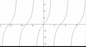
The second part of the exercise involved the students being asked to sketch graphs of six different functions. A breakdown of the students’ results is shown below:
|
Sketch a complete graph of the function |
% Correct |
|
|
|
|
52% 38% sketched a quadratic |
|
|
|
52% Ellipse—24%; figure not touching axes—24% |
|
|
|
57% |
|
|
|
5% General shape—57% |
|
|
|
94%. |
|
|
|
33% General shape—28% |
Fig. 3 shows a typical student solution to the question; sketch a complete graph of the function y = Ö(36 - x2). By looking at the keystrokes we can see exactly what the student did. Table 1 is a summary showing the results after a sequence of keystrokes.
Table 1: An example of the keystrokes of the student who drew Fig. 3
|
[Y=] |
[GRAPH] |
[ZOOM] |
[WINDOW] |
TBLSET |
TABLE |
OTHER |
||||
|
36 37 |
Ö(36-x2)) Ö(36-x2) |
32 38 40 42 |
39 |
|
31 41 |
-50,50,10, (-160, 60), 10 -25,25,(10), -1 ,6,1 |
|
|
33 34 35 43 |
Calc minimum Calc Value x=0-9 Calc Max x= -13.07. y=96.31 Trace – x=5.85 y=1.328 x=6.38 y= x=7.44 y= |
The numbers in the columns (e.g. 31, 32) represent the outcomes of such a sequence. For example, the sequence 36 results in the function y = Ö(36 - x2) being entered into the Y= screen. The student immediately pressed GRAPH (sequence 37). Because he had not changed the window settings from the previous question what he saw was a small horizontal line close to the x–axis. He next pressed the ZOOM button but decided not to do anything with the zoom and pressed graph again. His next step was to set the window shown in sequence 40 and press GRAPH. He then proceeded to trace along the curve the calculator had produced. The screen he saw is shown together with the sketch he made in Fig. 2. As we can see the student copied the calculator screen directly onto his answer sheet. There were many other examples like this one.
|
|
|
|
Fig. 3: Student sketch together with the calculator screen shot of the function
|
|
What we see from this and many other examples of the students work is that their basic knowledge of functions and their graphical representation is weak. A question we should ask is ‘Has the use of the graphic calculator contributed to this?’
5 Observations
The working styles adopted were predominantly
Trial
and alteration.
Using
the calculator for checking.
Many
just copied the calculator screen.
On
the first set of questions not one student set the calculator window similar to
the scale in the question.
The
majority of the students having entered the function just hit the graph button,
thus using the window settings for the previous function.
Several
students remembered what they had previously been taught and used calculus to
help with the sketching. However it was interesting to note that on at least
two occasions, when they identified stationery points they did not include them
on the sketch, they just copied the calculator screen.
6 Discussion
Having designed and evaluated the key recorder software, we are now exploring ways that such software can be used. An obvious interest is the extra insight that can be obtained from using such software because we can study exactly what the students are doing and this should enable us to deduce their understanding of the mathematical concepts. The fact that the students are unaware that they are being recorded means that they will be using the calculator as naturally as possible. The software will also give us the opportunity to investigate how a student uses the calculator outside the classroom.
The insight it gives us should enable us to develop ways of best practice. For example, the apparent failure by many of the students to set an appropriate viewing window when drawing a graph with a graphic calculator led us to devise the following algorithm to assist students when drawing a graph. It should be stressed that this algorithm is primarily for the inexperienced user of a graphic calculator.
|
|
|
|
|
Fig. 4: An algorithm for drawing a graph using a graphic calculator |
||
One important point to note is that as with computers, students are likely to adopt a button pressing experimental strategy to solve problems. So that teaching / learning materials produced for the graphic calculator should encourage students to regularly write down what they have discovered. This should encourage them to reflect on what they have been doing.
Anybody who wants further information about the software or who may be interested in working with the team at Plymouth, please contact jberry@plymouth.ac.uk .
References
Finney, R.L., Thomas, G.B., Demana, F. and Waits, B.K. (1994) Calculus: graphical, numerical, algebraic. Addison-Wesley, New York.
Penglase, M. and Arnold, S. (1996) The Graphics Calculator in Mathematics education: A Critical Review of Recent Research., Mathematics Education Research Journal 8(1), 58-90.
Ruthven, K. (1990) The Influence of graphic calculator use on translation from graphic to symbolic forms., Educational Studies in Mathematics 21(5) 431-450.
Thomas, P. and Paine, C. (2000) How students learn to program: observations of study time behaviour. Research Report 2000/2. Computing Department, Open University, Milton Keynes, United Kingdom.
Weigand, H-G. (1999) Evaluating working styles of students in a computer based environment. Proceedings of the fourth International Conference on Technology in Mathematics Teaching. University of Plymouth, Plymouth, United Kingdom.
Diagnosing mathematical needs
and following them up
Neil Challis, Harry Gretton, Michael Robinson, and Stephen Wan
Sheffield, UK
2. A cameo of mathematical diagnosis activity in the UK
4. Follow up support structures
5. The role and impact of technology
1 Introduction
The UK higher education system is in a state of flux, and has been for some time. Entrants to university are more diverse. There has been evolution in school level mathematics to which some university disciplines, which are „users“ of mathematics, are struggling to adjust. There is a decline in numbers of students wishing to study technical subjects at university level. There is a general perception of a declining level of traditional mathematical skill and knowledge in the narrow sense on entry to university (e.g. Engineering Council (2000), Croft (2001)), although new students frequently do possess other qualities, for example a good level of IT skill, which their predecessors may not have possessed.
Within this context, there is recognition that we can no longer assume the same level of homogeneity as even 15 years ago concerning the prior mathematical experience of students arriving on our courses. A significant proportion are mature students, but in any case prior experience may include A level, AS level, vocational qualifications, foundation or access courses, or overseas qualifications. One response to this is the current interest in diagnosing mathematical baggage and initial needs of these diverse entrants to university.
In this paper, we describe a current project at Sheffield Hallam University, addressing mathematical diagnosis and follow up. This is not new work; it is volatile, continues and develops, and makes more concerted our previous work in this area (e.g. Challis and Gretton (1997), Challis and Gretton (1998)). We try to find out, at the initial stages of a course, what kind of academic support students need in mathematics, by trying to identify what they already know or can do in topics relevant to their course. Groups involved in our work include some six hundred first year undergraduates in engineering, the built environment, the sciences, mathematics, business and technology. There is some diversity here both in the students recruited, and in the requirements concerning mathematics on the various courses.
We begin by presenting the qualitative results of an informal survey of diagnostic and follow up activity in UK universities, which we have carried out with the aim of looking at existing practice. We then describe in a little more detail our current developmental work, and include discussion of the general educational issues, for instance around curriculum design and student support mechanisms, which are raised by these activities.
We present this work at a conference concerning technology in mathematics teaching, since some would see technology as having a major role in addressing the issues raised above. We discuss later the influence of technology on this work.
2 A cameo of mathematical diagnosis activity in the UK
The survey, of universities chosen after literature and Internet searches, was carried out mainly through telephone interviews, with a few responses via email. For this small project, a limited informal and qualitative approach was deemed suitable. (Wider work is being focussed through the UK’s national subject centre in Mathematics, Statistics and Operational Research (LTSN Maths, Stats and OR Network, 2001), and more thoroughgoing work commissioned by that body will be reported in the near future.) In this current work, eighteen academics were surveyed from sixteen different universities, fifteen were interviewed via the telephone, three responded via email. Key questions related to:
the
nature of mathematics provision at the university and the academic’s role in it
reasons
for using or not using diagnostics
the
nature of any diagnostics used (paper-based versus computer based etc.)
the
quality of feedback provided and the nature of follow-up support provided
Fifteen of the academics interviewed were responsible for the teaching of level one undergraduate mathematics, service or otherwise. Three were either heavily involved in the design of a computer based diagnostic or they managed a central mathematics support centre for their university.
The ten academics using some form of diagnostic generally believed that this is required to meet the challenge of teaching increasingly diverse entrants. Their most common reason for implementing diagnostics was that prior formal qualifications do not provide sufficient indication of a student’s mathematical competency. In contradiction, the main argument cited for not using any form of diagnostic (other than those who said they faced logistical and resourcing issues) was the fact that A-level grades in particular were adequate indications of student competency levels! These latter universities were, however, those, which enrol students that on the whole have obtained good A-level grades.
Of the ten academics who used diagnostics, five used a paper-based form whilst five used a computer-based form. Those who used computer-based diagnostics argued that the main advantages were time efficiency, automatic marking and instant feedback for student and tutor. These computer-based diagnostics were developed either in-house or by another university. Of those computer-based diagnostics cited, only ‘Diagnosys’ (Diagnosys, 2001) appeared to offer something over and above paper-based versions. Diagnosys is a knowledge based diagnostic tool that can be customised in its approach, taking into account the student’s mathematical background or stated course of study and also the correctness of the previous question in determining an appropriate following question. It was argued that teaching and learning could be directed in a specific and effective manner using this software. However, no evidence or evaluative data was offered to support this claim. The nature of follow-up support for students at universities that used Diagnosys did not appear to be markedly distinct from those who said they used other computer-based or paper-based diagnostics. Furthermore, there did not appear to be much difference in the approach to follow-up support by those who used computer-based and those implementing paper-based diagnostics.
There was a wide array of follow-up support activities amongst the universities surveyed. Five universities have operated some form of mathematics support centre. All of these universities implemented some form of diagnostic, sometimes instigated by staff in the support centre rather than course leaders. Follow-up support by these universities was heavily reliant on students voluntarily seeking support with their mathematical skills in light of diagnostic results (usually obtained before formal teaching started). Staff at mathematics support centres offer drop-in sessions for one to one tutoring and are able to offer worksheets, computer based tutorial packages and revision material. Virtually all of the academics mentioning their mathematics support centre were concerned that they were not reaching those students who were most in need of support. It was often said that students attending were perhaps not necessarily weak in their skills but simply lacked confidence.
Supplementary classes were a common method of addressing follow-up support needs. These varied from compulsory attendance (some called these «remedial» classes) by those either under-performing in diagnostic tests and/or directed by virtue of their lower prior qualifications. Non-compulsory supplementary classes were often used to target students who were diagnosed with a weakness in particular areas of mathematics. The rationale for non-compulsory classes was that it encourages students to take ownership of their learning. A tactic employed by a few universities for further encouragement, is to allocate a certain topic to certain weeks of the semester, so that students are able to target their attendance to classes according to their perceived areas of weakness. Both forms of supplementary classes are said to have their problems. Compulsory classes were said to be counter-productive, not only by stigmatising students, but also because it could be used as an excuse for students to reaffirm their inability to master the fundamentals of mathematics. Staff who run non-compulsory classes on the other hand, complain of attendance dropping off week by week.
Streaming of students according to mathematical background and qualification was used by a number of universities, instead of a diagnostic, although a couple of universities used a form of streaming based on diagnostic results. It was commented though that this raised a prevailing issue of equity, where students are required to study for the same number of credits and undertake the same amount of work on the same courses.
Other methods of tackling this issue included the use of information packs sent to students (e.g. revision material) a few weeks prior to their university course with the intention of encouraging students to brush up on their mathematics. A couple of universities integrated «diagnostic» testing as a small part of the assessment at level one, but their aim was to encourage students to engage with their mathematics rather than to diagnose. Two universities mentioned revising the syllabus. One academic explained that some higher-level material had been replaced by more suitable content for today’s students, whilst another explained that the mathematics provision for students on certain courses had been extended from two semesters to three semesters.
Overall, the survey did not indicate a common practice in diagnosing the mathematical needs of students across the UK universities, there does not appear to be a consensus as to what diagnostics can achieve, and there is great variability particularly in the area of supporting students. Furthermore, the survey did not elucidate any real evaluation of the value of implementing diagnostics or effectiveness of follow-up support. The feedback from this survey has informed both positively and negatively the progress of our own project.
3 Why diagnose?
The first stage in our own two stage process is to aim to diagnose student need preferably in week 0, using a set of diagnostic questions set on the web, but avoiding using the T-word (test), although not all are as squeamish about this as we are. It might be informative to begin this section by considering critically various reasons given for using a diagnostic test.
«You can assess overall standard to identify the appropriate level for the group.»
«You can assess any change in entry ‘standards’»
Within the immediate educational aims of our project, these reasons are not relevant. Regardless of one’s opinion concerning any perceived longer-term change in UK A-level or other standards, it is clear that natural year-on-year changes are small, except where there has been an explicit change in curriculum, about which we should know anyway. A one-off diagnosis cannot say anything helpful in this respect. Adjusting to minor differences from year to year should be relatively easy for lecturers and tutors who are aiming to take into account the prior experience of their students. In the longer term, it is perhaps in any case not reasonable or even desirable in a rapidly changing and increasingly technological world to expect students to arrive at university with the same skills and knowledge as we had when we arrived 10, 20 or 30 years ago. Indeed an attempt to turn the clock back can be counterproductive to the aim of persuading students to study mathematically based subjects.
«You can assess specific subjects which need attention for the whole group.»
Of course, what we do not get from a student’s entry qualifications is any indication of those topics with which students had difficulties. In terms of the whole group provision, again it seems unlikely that one-year’s cohort will be significantly different, on average, from its immediate predecessor. It follows that the lecturer will probably be able to decide which topics need to be covered and in what depth based on their recent experience of teaching similar students. That said, a diagnostic may alert the lecturer if they have not spotted a topic area, which is causing problems.
«The tutor can identify an individual student’s needs.»
«Students can identify their own needs»
The crucial issue for us in relation to diagnostics is the wide variation between individual students and what we do about it. Again it is worth noting here that if we want to identify the weaker students, their A-level or equivalent results might be the most appropriate means of doing this. It is tempting to assume that using a diagnostic (especially one designed in-house) is a more reliable indicator of the students’ abilities, but the case for this is not proven. This brings to mind the more general point concerning how well entry qualifications predict final results, but this is not the place to explore that further.
What a diagnostic test can indicate then (to tutor and student) is the current ability of a student in a specific topic, and thus which topics the student needs to work on. There are two points to be made here. One is that the word current is important: students arriving in September have done no mathematics, generally, since the previous June or even earlier. A student whose mark is poor in week one may show substantial improvement very rapidly if they are simply lacking recent practice. The second point is that the word ability needs some exploration. Most diagnostics go as far as testing the surface level of mechanical skill, but do not perform a deep analysis. For example suppose we ask a student to solve a quadratic equation. If they get it wrong, this could have been caused by ticking the wrong multiple choice box, arithmetic error, forgetting the formula, pressing the wrong button on their TI-8* calculator, a total lack of understanding of the «why» and «how» of quadratic equations, and so on. If they get it right, that could mean they can mechanically and correctly administer the formula or press the right TI-8* button, but their understanding of the topic may be shallow. This may be OK if all they need is the ability to perform «mindless symbolic manipulation».
In deciding then how far we think that a diagnostic can be useful, we question the long-term significance of any diagnostic administered at the start of term. Within a few weeks we would expect to have a clear idea of individual student needs from their performance in coursework, tutorials, and through talking to and motivating them. There is no substitute for observing the students in small groups, although small groups are a luxury not many can afford! We therefore see diagnostics primarily as just one piece of evidence to help us identify that a student is in need of extra support in the very first few weeks of the first term, and importantly to help the student to realise this for themselves. The lack of exploratory depth in the diagnostic is not then a problem; a deeper process of analysis of a student’s understanding is more properly part of the ongoing educational process.
Because of the limited usefulness of diagnostics, we feel disinclined to spend a great deal of time and effort in designing the perfect diagnostic; there is no such thing. Their use is mainly in the first weeks of term, and it is vital that we get the results as rapidly as possible. We therefore choose a very simple computer-based multiple-choice diagnostic, using existing web-based technology, which can allow instant, crude yes/no feedback both to students and to lecturers. This diagnostic is quick to take and can be done in the first one hour tutorial. Given the limitations on the depth of the analysis (imposed by the constraints of time and technology), the main result of the diagnosis can be said to be that it forms a «conversation piece», something to initiate the process of mathematical education, of reflection and action planning, and certainly not a once and for all analysis of a student’s base skills.
4 Follow up support structures
Before going on to describe various remedies we apply, there are two general points to be made concerning following up on the diagnosis. The first concerns student take-up of what is on offer – some will take advantage of it and some will not. How do we encourage people to do what they should? The question of how we motivate students in a mass higher education system is one which many university lecturers brought up in an elite system have not had to face before: it is of course easier to motivate students in smaller groups, where there is no hiding place! The second point is that there is not one response, which fits all, because of the diversity of students, of courses, and of resources. Thus our response is diverse, but one constant is that we do not ever use the R-word (remedial).
All students can use «Maths Help» and all students can access a range of resources.
Maths Help is a drop-in session, which runs for 2 hours daily all year, is open to all students and staff, and is regularly identified as highly popular with students in internal and external quality reviews. The main problem is satisfying demand within the limited resources for running the session. We also have a resource base of materials created here and elsewhere, and are currently collating a range of internal materials to be made available on the web. We are designing web-access to the resources, which makes it easy for lecturers to add material, and easy for students to find things.
Some materials consist of fairly recently designed computer based learning (CBL) packages such as Mathwise (Mathwise, 1999), and indeed the use of such packages is presented by some as the cheap solution. However, upon evaluating, we have found some difficulties. Most students will not go away and use such a package unless under supervision; students have been observed to just press buttons - that is, superficially flicking through pages and multimedia activities without engaging in the material; and it is not uncommon for students to print out every page to work at later, and to keep a record, negating the benefits of live activities. We might observe here that the philosophy of «testing» a group, and then sending the «weaker» students to a CBL package is fundamentally flawed anyway. It is a conclusion from our experience that these students are precisely the ones who need human contact over their mathematics to help them to build confidence and to keep them motivated!
Some students, for instance in science and mathematics, have some degree of free choice and can attend extra elective units, the content of which can in part be formed by the diagnosis.
We have credit carrying elective units called Maths Workshop 1 (assuming a low level of previous mathematics) and Maths Workshop 2 (assuming below average previous mathematics), designed to increase confidence levels in mathematics, allow extra time for practice, and look at some mathematical topics in a broader way than pre-university. A diagnostic is used as one indicator, alongside prior results (or lack of them) and the student’s own preference, in selecting, which unit students should take, or whether to take neither. The diagnostic results will inform the starting point for individual students.
Some students, for instance in engineering or the built environment, are allowed extra contact time within their mathematics units if they are identified as needing it
We have previously provided extra contact time for some students. Last year some students were advised to make use of this, although take up was relatively low, and the issue of motivation arose. The sessions appeared popular with those students who did attend. They included some drop-in; some ‘chalk and talk’ covering material perhaps in a different way; and some identified students working on tutorial sheets/assignments and seeking help. One way in which students were identified as in need was that they were registered on a diploma rather than a degree course. It turned out that this was not a good indicator, and perhaps a better one would be some measure of level of motivation and enthusiasm!
For next year we plan to provide a more structured and possibly more varied support set-up. For example we may include structured workshops on specific topics (e.g. telling students that weeks 2 - 5 will be on a basic algebra, and weeks 6 – 8 will be on calculus, etc.). The theory here is that students are more likely to attend if they know that a session is particularly relevant to them.
5 The role and impact of technology
The impact of technology is felt throughout mathematics, and the activities we are describing here are no exception. In fact technology raises some fundamental questions concerning what we are doing. First there are some purely practical and not original points. The diagnostic results must be provided instantly for maximum educational impact, and so a web-based diagnostic is best. The rough and ready nature of what we propose to use means that multiple choice is adequate for the purpose, although of course this would not be so if we were aiming for a deeper analysis. However practical concerns can intrude here, such as network reliability, and logistic difficulties, and so we hear that some people have reverted to paper based diagnosis marked by an optical mark reader.
A second, philosophical, issue arises during follow up, upon which we have already commented, concerning the educational limitations to the role which can be played by CBL packages.
Finally there is a fundamental point at which we have hinted earlier. This concerns the changing nature of «doing» mathematics as technology develops (e.g. Gretton and Challis, 2000). In rapidly changing times such as these, with computer algebra systems, spreadsheets, dynamic geometry packages, and powerful and inexpensive hand-held mathematical technology such as the TI-89, we would not expect the curriculum on any course to be set in stone. There is much talk of falling standards, but surely maintaining standards cannot be treated as synonymous with making things the way they were when we were undergraduates. In this present context, this means we must work out what questions we should be asking in any diagnosis, but of course the prior question is what mathematical ideas and practices we should be valuing by having them in our curriculum. Technology is a key influence on the answer to this.
6 Evaluating the work
Although we have been operating a variety of diagnostics for some time, this project aims to make our approach more concerted, with shared good practice within a diversity of tactics. We thus plan to evaluate what we are doing in the course of the next year. A scientific «control group» approach is not appropriate, and the evaluation will take the form of semi-structured interviews with a range of students and tutors both individually and in groups. We are particularly interested in how students may integrate this activity through skills portfolios which some construct. This work encourages self-assessment and self-identification of needs, has been the subject of previous work with engineering students (Challis and Gretton, 1997), and is being implemented with mathematics students next year.
7 Concluding remarks
We keep our concluding remarks brief, and leave the reader with just three questions.
We are attempting to use a rough and ready diagnosis to help along the educational process with students. Should not that be part of what we are doing all the time?
We have deliberately not listed the topics, which are the subject of our diagnosis. We raise again not only what are the topics that we should be diagnosing, but the broader question of what mathematics we should be teaching in a technological age.
Finally we note that it is fashionable in the UK to talk about the Mathematics Problem. Our concern here is that this kind of language gives the impression that mathematics is in a bad state, instead of being a wonderful, exciting and useful subject to study. Who has the problem?
References
Challis N.V. and Gretton H.W. (1997) Technology, key skills and the engineering mathematics curriculum. Proc. 2nd IMA conference on Mathematical Education of Engineers, IMA, Southend, 145-150.
Challis N.V. and Gretton H.W. (1998) Learning diaries and Technology: their impact on student learning, Proc. ICTMT 3, Institut fur Mediendidaktik der Universitat in Koblenz, CD-ROM, Koblenz, Germany.
Croft A C. (2001) Following up cycles of QAA subject assessments for non-mathematicians. MSOR Connections 1, 2, 17-18.
Diagnosys, 6 March, 2001, The Diagnosys homepage,
http://www.staff.ncl.ac.uk/john.appleby/diagpage/diagindx.htm
Engineering Council (2000) Measuring the Mathematics Problem, Eng. Council, London.
Gretton H. W. and Challis N. V. (2000) What is doing mathematics now that technology is here? Proc 5th Asian Technology Conference in Mathematics, ATCM Inc, 285 - 293
Maths, Stats and OR network, 25 June 2001, LTSN Maths, Stats and OR network,
Mathwise, 13 April 1999, The UK Mathematics Courseware Consortium, Mathwise,
http://www.bham.ac.uk/mathwise/
The impact of training for students
on their learning of mathematics
with a graphical calculator
Roger Fentem and Jenny Sharp
Plymouth, England
1 Introduction
Much of the research outcomes and findings into the impact of the use of graphical calculators on students’ achievement in mathematical assessments (Bridgeman e.a., 1995), on students’ conceptual understanding (Shoaf-Grubbs, 1993; Smith, 1997) and students’ attitude to studying mathematics (Berry e.a., 2001; Nimmons, 1998) have been largely positive. Dunham (2000) sites a “few instances” where calculator usage resulted in negative outcomes in respect of conceptual development. These research studies are characterised by treatments of short duration. Streun, Harskamp, and Suhre (2000) investigated the duration of usage and observed that students exposed to prolonged use (at least a year) outperform, have a richer solution repertoire, and have a better understanding than those with more limited exposure.
Heid (1997) raises the issue of designing the teaching material with technology in mind. Dunham’s research perspective (2000) highlights the importance of fully integrating the technology “as a standard tool available to all students as a part of regular instruction.” These bring into sharp focus the crucial role of the teacher in students’ learning of mathematics. Doerr and Zangor (1999) found three aspects of the teacher's role, knowledge, and beliefs that contribute to the development of support of their students’ learning of mathematics. These were (i) the teacher's confidence and flexible use of the tool, (ii) the teacher's awareness of the limitations of the technology, and (iii) the teacher's belief in the value of the calculator to support meaningful investigations. Teachers’ beliefs about the nature of mathematics, their attitude towards changes in teaching (classroom) practices, and the potential of graphing calculator technology to produce the desired learning outcomes (Futch and Stephens 1997; Simmt, 1995; Tharp, Fitzsimmons, and Ayers, 1997) have all been featured as being important considerations. One conclusion of the research review conducted by Penglase and Arnold (1996) was that “Teachers and students who know little or nothing of graphics calculators will most likely be reluctant to use them, and certainly will not be able to utilize their full potential.”
Simonsen and Dick (1997) examined In-Service training and support for teachers I the use of graphing calculators. Porzio (1997) concluded that students behave as they are taught. In a large scale study, Lagrange (1999) reinforces the view that teachers need to support students in their learning mathematics through the use of calculators: “… teachers must control students’ development of utilisation schemes and their co-ordination with the advancement of mathematical knowledge.”
The findings from over a decade of use of graphing calculators reveal the complex nature of the interaction of technology and teaching in the learning of mathematics. It is clear in this that graphing calculators can have, given time, a positive effect on students and that teachers need support in incorporating the technology into their teaching. What effect does the training of students in the use of the technology have? It is this question, which is at the heart of the investigation we have started.
2 Research aims
This paper introduces a longitudinal (two years) research project designed to investigate this issue of technology training for both teacher and student in studying mathematics post 16. Attitude, relative achievement, and practice are studied, recorded and analysed.
One class of 16-18 year old mathematics students in each of four schools in the UK have been provided with the same graphing calculator for their use throughout the two years of their course. A teacher in each school is also provided with the same calculator and a means of projecting the image of the calculator screen to the whole class for instructional purposes. The teachers in two schools had previously had training in graphing calculator technology (using a different make of machine), the teachers in the other schools had not.
The students from one school in each of the two groups of schools receive focussed, on-going training in graphing calculator use and functionality. All students and teachers keep a regular log of their use of the technology in mathematics classes. The attitudes of the students on learning mathematics with technology are analysed. Their relative achievements, in national examinations, using prior success in national examinations as a value-added indicator are measured.
All the students in the study are preparing for the same set of examinations and initially are being prepared for the same examination at the same time. The General Certificate of Education (GCE) Advanced level in Mathematics consists of six modules in which the examinations are externally set and marked. In two of these modules (P1, P2) students are restricted to the use of a scientific calculator and in four of the modules students may use a graphing calculator. The first module examination taken by all the students is P1. They sit this examination approximately six months after embarking on their GCE studies. Other modules are sat after one year, eighteen months and two years of study.
All students have taken a set of GCSE examinations at age 16. In this portfolio of examinations, they all sit Mathematics, English, and Science. They then have some measure of choice of up to 7 other subjects. Their outcomes in these examinations are to form the value-added indicator.
The following diagram intends to present a time-event picture of the study:
|
Time |
Event |
||
|
Summer 2000 |
GCSE outcomes |
|
Ongoing log |
|
Autumn 2000 |
Commence GCE |
|
|
|
January 2001 |
P1 module examination |
Attitude questionnaire |
|
|
Summer 2001 |
P2 + possibly other module examinations |
|
|
|
January 2002 |
Other module examinations |
|
|
|
Summer 2002 |
Final module examinations |
Attitude questionnaire |
|
It is intended that the structure of the research design will allow the impact and extent of training, at both teacher and student level to be investigated. There are four levels of exposure to training: both teacher and student trained, only student trained, only teacher trained, and neither student nor teacher trained.
|
|
Student |
||
|
Trained |
Not Trained |
||
|
Teacher |
Trained |
ü |
ü |
|
Not Trained |
ü |
ü |
|
3 Findings
Much of the activity to date has focussed on producing and delivering appropriate technology training for the students. Attitude questionnaires have been administered, logs have been returned by teachers and students, and students have sat examinations. Analysis of data has yet to be commenced.
References
Berry, J., Fentem, R., Partanen, A.-M., Tiihali, S. (2001) Hand-held Computer Algebra Systems and calculators: Students Attitudes and Beliefs in their use in Learning Mathematics (in preparation).
Bridgeman, B., Harvey, A. and Braswell, J. (1995) Effects of calculator use on scores on a test of mathematical reasoning. Journal of Educational Measurement 32, 323-340.
Dunham, P. (2000) Hand-held calculators in mathematics education: a research perspective. NCTM Year Book 2000.
Futch, L.D. and Stephens, J.C. (1997) The Beliefs of Georgia Teachers and Principals Regarding the NCTM Standards: A Representative View Using the Standards’ Belief Instrument (SBI). School Science and Mathematics 97(5).
Heid, M.K., (1997) The Technological Revolution and the Reform of School Mathematics. American Journal of Education 106, 5-61.
Lagrange, J.-B. (1999) Complex Calculators in the Classroom: Theoretical and Practical Reflections on Teaching Pre-calculus. International Journal of Computers in Mathematical Learning 4, 51-81.
Nimmons, L.A. (1998) Spatial ability and dispositions toward mathematics in college algebra: Gender related differences. Dissertation Abstracts International, 58, 8.
Penglase, M. and Arnold, S. (1996) The graphics calculator in Mathematics Education: A critical review of recent research. Mathematics Education Research Journal 8, 1, 58-90.
Porzio, D.T. (1997) Examining Effects of Graphics Calculator Use on Student Understanding of Numerical, Graphical, and Symbolic Representation of Calculus Concepts. Annual Meeting of the American Educational Research Association (Chicago).
Shoaf-Grubbs, M.M. (1993) The effect of the graphics calculator on female students’ cognitive levels and visual thinking. Dissertation Abstracts International 54/01, 119.
Simmt, E. (1997) Graphing Calculators in High School Mathematics. Journal of Computing in Mathematics and Science Teaching 16, 269-289.
Simonsen, L.M., Dick, T.P. (1997) Teachers' Perceptions of the Impact of Graphing Calculators in the Mathematics Classroom. Journal of Computing in Mathematics and Science Teaching 16, 2~3.
Smith, B.A. (1997) A meta-analysis of outcomes from the use of calculators in mathematics education. Dissertation Abstracts International 58, 787A.
Smith, K B and Shotsberger, P. G. (1997) Assessing the Use of Graphing Calculators in College Algebra: Reflecting on Dimensions of Teaching and Learning. School Science and Mathematics 97(7).
Streun, A. von, Harskamp, E., and Suhre, C. (2000) The effect of the graphic calculator on students' solution approaches: a secondary analysis. Hiroshima Journal of Mathematics Education 8, 27-39
Tharp, M.L., Fitzsimmons, J.A. and Ayers, R.L. (1997) Negotiating a Technological Shift: Teacher Perceptions of the Implementation of Graphing calculators. Journal of Computing in Mathematics and Science Teaching 16, (4), 551-575.
Data collection and manipulation using
graphic calculators with 10-14 year olds
Ruth Forrester
Edinburgh, UK
1 Introduction
A teacher researcher group at the Edinburgh Centre for Mathematical Education is currently investigating the use of graphic calculators in Mathematics classes for pupils aged 10 –14 years. Graphic calculators are now widely used in Scotland in the teaching of Mathematics to students aged 16+ and most teachers agree that they are a valuable tool at that level. Their use is, however, limited by the time required for pupils to learn to operate these machines. The research group has focussed on the 10 –14 age group, investigating the possibility of fruitful Graphic Calculator use at this earlier stage. Classroom resources have been developed and their use investigated in a variety of different classroom situations. (Forrester and Searl, 2000; Forrester, 2000).
One aspect of this work has been an investigation of the possibilities graphic calculators may offer in the development of data handling skills. The calculators used are the Texas Instruments TI 73s which were designed particularly for top primary / early secondary pupils. These are easier to use than the more sophisticated machines designed for older students but they offer facilities for some fairly advanced statistical calculation and plotting.
Data handling skills are increasingly important in society. For example, this has been recognised by the introduction of statistical content in the Scottish school curriculum. Information handling attainment targets at level F of the National Guidelines for Mathematics 5–14 specify that pupils should be able, in the course of Primary 7 or in the first or second year of secondary school, to:
Collect
information using practical experiments, surveys and sampling;
Organise
information by grouping and ordering discrete / continuous data;
Display
information by constructing stem and leaf graph, scattergraphs, piecharts;
Interpret information by retrieval from
displays and databases, by describing correlation in scattergraphs in
qualitative terms and by calculating mean, median, mode and range of data sets.
(SOIED, 1999).
Pupils will benefit from learning how to operate graphic calculators in this context and how to use them as ‘black box’ technology to ‘get answers’. Facility with hand held technology will benefit pupils in their future studies. Statisticians use technology to manipulate data. ‘Button pushing’ skills may also be transferable to computer packages and new data handling technologies yet to be invented.
More important, however, is an investigation of the potential of graphic calculators as tools to facilitate the development of pupils’ understanding, not just to ‘get answers’. A series of activities was devised for classroom use. Pupils would perform the experiments and make measurements to collect a large amount of data about the class members. The data would be collected on record sheets, entered into lists on the graphic calculator and then analysed appropriately.
The experiments and measurements were mainly adapted from tests used by doctors in medical check-ups. The data to be collected was:
Gender
of pupil
Eye
colour
Age
in days
Day
of week of birthday this year
Height
Length
of right foot
Distance
pupil can blow 1p across a desk
Score
when blu-tak is dropped onto a target ( 0 (miss) to 8 (bullseye) )
Length
of time pupil can hold breath
Volume
of water drunk in one suck
Number
of steps (up and down) in 1 minute
These measurements / experiments were piloted by a Primary 7 class (11-year-olds). This resulted in some modification of the record sheet to remove ambiguities and a simplification of the process of entering the data on the graphic calculator. The teachers in the group were concerned about potential difficulties caused by individual pupils keying their own data into the correct lists. It takes time to learn how to operate lists and it would be very easy for one student to accidentally delete or mix-up other entries. It is also difficult for the teacher to detect errors. Simple programs were used to help pupils key their results into the lists without having to learn in detail how to operate lists on the TI 73. The programs also put the entries into order according to the record number.
2 Classroom implementation
These data collection activities were used with a Secondary 2 class of 13-year-olds attending a comprehensive school in Edinburgh. A substantial database of information about the class members was assembled during the first session. One week later the class worked with the database using the statistical plotting facilities of the TI 73. A ‘stations’ approach was used for the collection of data. One calculator, running the appropriate program, and the necessary equipment were placed at each station. Pupils were divided up into small groups and each given a record number. At each station the group carried out the experiment and members entered their own data onto their individual data sheet and into the calculator with their record number as prompted by the program.
The process of collecting the data offered considerable opportunity for collateral learning. Pupils were forced to consider the kinds of difficulties that may be faced when collecting real data. Rules had to be negotiated by the group so that results could be compared fairly. (For example, how far above the target should the blu-tak be held before dropping? Can pupils have a practice shot? Did everyone take their shoes off to measure foot length? What about thick socks?) Issues of measurement became important to the pupils. (Which side of the coin should be measured to? How accurate should the measurement be – to the nearest centimetre or to 1 decimal place?)
The programs were effective in entering data into the lists in order and in preventing pupils from interfering with previously entered data. There were errors – missing and double entries were the main problems - and simple checking programs have subsequently been produced. These highlight such entries along with any data outside an expected range. This helps the teacher to make corrections efficiently using the data record sheets. After corrections were made the lists were all copied onto one calculator ready for analysis in the second session.
The analysis and graphing of the information gathered was performed on just one calculator using an overhead projector. While pupils’ involvement with the data is important, teacher input is necessary at this introductory stage and so a whole class approach was adopted. During the lesson, pupils were asked to sketch graphs before they were drawn on the calculator. They were asked to make suggestions for the window settings and to predict the shape of the graph in each case. These predictions were then discussed with the class as a whole and pupils’ suggestions for maximum and minimum values on the axes used to draw the graphs. This process had the advantage of providing a record of pupils’ thinking as well as actively involving them in the lesson.
Pupils were clearly interested and involved in the lesson. The technology played an important part in this. There was an audible “ohh” when the first graph came up on the screen. Students were keen to suggest new graphs to try and the facility to draw and redraw the same graphs with different scales was very effective especially when pupils had different opinions about what the scales should be. The teachers involved were impressed by the way in which the lesson held the students’ attention for the full hour (especially since pupils did not operate the calculators themselves). The fact that the pupils’ own data was used also had a motivating effect. Pupils were very keen to look at the data in the lists and pick out particular people.
Pupil: “That was me”
Pupil: “I was on a Tuesday”.
There was great interest in seeing the data referring to one particular boy (Gary) who is very tall.
|
|
Jo-Ann picked out the point referring to Gary on her scatter graph plotting height against foot length. |
|
Fig. 1 |
|
|
|
Another pupil drew a separate bar for Gary on the histogram showing heights: |
|
Fig. 2 |
|
Pupil (excited): “That was Gary 1·95. It had to be.”
The class were also very anxious to pick out the data and position on the graph relating to another boy (Murray) who drank almost all the water in one suck.
Pupil (excited): “Miss Robertson, you said somebody drank all the water….somebody got 100mls.”
There was particular interest in the scatter graphs comparing the “steps” (and then “foot length”) of the boys with those of the girls.
|
|
Fergus predicted that all the boys would make more steps up and down in one minute than any girl. |
|
Fig. 3 |
|
When pupils were deciding on suitable axes for the graphs, they were able to refer back to their experience of making the measurements to help choose sensible scales. For example, when suggesting suitable axes for the histogram of eye colour, one pupil suggested 0 to 15 because they thought there would be no more than half the class in each group. Another pupil chose 0 to 20 because they thought there would be a lot of brown eyes. They also used the data lists on the calculator.
Pupil: “Can we see the list again, Miss?”
Although corrections had been made to data wrongly entered, the learners were able to appreciate some of the difficulties of dealing with real data (eg. missing data entered as zero and the effect of this on the resulting graphs).
|
|
Andrew predicted a ‘normal’ curve but then modified his diagram to show more missing entries. |
|
Fig. 4 |
|
Some pupils were able to come to a fairly sophisticated appreciation of the effect of changing the interval grouping of data on the resulting graph. The graphic calculator was an ideal tool in this situation – instantly able to illustrate the effects of different interval groupings.
Discussion of predicted histograms for ‘steps’ experiment:
Pupil: “Do you not put it in intervals here?’
Teacher: “Yes, we can’t have a different bar for each number, can we? Because we’d have about 60 bars or something…. So how could we overcome that?’
Pupil: “Put 0 to 20 and then 21 to 40 and 41 to 60.”
Teacher: “Groups of 20 at a time.”
(Another) Pupil: “No, 10 at a time.”
Teacher: “Let’s try both. We’ll start with 20 and then try it again with 10 and see if it makes a difference.” (Discussion about Y scale and shape of graph expected. Pupils predict normal curve).
Teacher: “Let’s graph it and see then.”
Teacher: “That didn’t go up to a maximum and back down again.”
Pupil: “Just went up to a max.”
Teacher: “Why’s that then?”
Pupil: “Because it went up in 20s, you’re going up in…..”
Pupil: “Taking big jumps.”
Pupil: “21 to 40 and then 41 to 60, it’s too big.”
Teacher: “Too big a group of people all put together in the same bar. Yes.”
Pupil: “Most people will get in between 50 and 60, not many people will get….” (unclear)
Teacher: “I’ll change the windows and instead of grouping them in 20s, I’ll group them in 10s. Would that do?….Aha, yes, just as you said.” (Discussion – decide to try groups of 5).
Teacher: “How do you think the shape will look?”
Pupil: “High between 60 and 64.” (Graph drawn)
Teacher: “Of course they’re not going so high because there’s less people in each little group.”
The work on histograms helped many students to understand when they should expect a normal curve and when they should not. For example, Arran and Heather (below) predicted normal curves when graphing the height of class members, the length of time they can hold their breath and the amount of water they can drink in one suck. They both realised that that the histogram showing which day of the week pupils’ birthdays fall on would not have a normal shape.
|
|
|||
|
|
||||
|
Fig. 5 a, b |
Fig. 6 |
Having a lot of data and the facility to be able to draw a variety of graphs quickly helped the teacher to guide pupils’ thinking about when and why a graph would take the form of a normal curve.
Discussion of predicted histogram of results from “steps” data:
Pupil: “It’ll sort of go up and …. Sort of at the top, it’ll go down.”
Teacher: “Why do you think it will go up and then down again? Will they not all be the same?”
Several Pupils: “No” (firmly).
Pupil (hesitating): “There’ll be quite a lot of people that’ll get one thing… then it’ll go off a bit…. and there won’t be very many people that get the other one.”
Teacher: “So there won’t be very many people that get an awful lot. There won’t be many 70s and 75s or 80s, right? There won’t be very many zeros and 10s but,…is this what you’re trying to say?… but there’ll be an awful lot of something in the middle.”
Pupil: “Yes, yes.”
Teacher: “Let’s graph it and see then.”
Discussion of histogram of height:
Teacher: “Did you get the shape? Did everybody say they thought there’d be a lot of people with a medium kind of height?”
Class: general agreement.
Discussion of histogram of day of week of birthday:
Teacher: “Can anybody predict for me, if I did a graph of what day of the week your birthday was, can you tell me what shape the graph would be?
Pupil: “All scattered.”
Pupil: “All scattered, all up and down.”
The class had some previous experience of scattergraphs. The use of the graphic calculator provided an opportunity for pupils to look at a variety of scattergraphs, some looking very different from those they had seen before. Pupils appeared to expect a general scattering of points probably distributed roughly along a straight line. Pupils found it difficult to predict the appearance of the graph plotting gender against foot length (despite prompting by the teacher to think about the position of the mark relating to each individual). Most were very surprised when the graph was drawn but were then able to correctly predict the shape of the graph plotting gender against steps.
|
|
|
|
|
|
|
Fig. 7 a, b |
Fig. 8 a, b |
|
|
|
|
Fig. 9 a, b |
|
The unexpected shape of these graphs pushed pupils to think more carefully about the significance of the placing of each point and pupils were able to appreciate that scatter graphs can look quite different from the ones they had seen before.
3 Conclusions
Small amounts of data can be collected and analysed by hand, (and this is a valuable experience for pupils) but interpretation of information from displays and databases does require technological support. The technology allows learners to deal with an amount of data large enough to make statistical analysis and plotting meaningful since it helps to make sense of the lists of figures. Pupils can handle real data in the way that statisticians do. This promotes deeper understanding of statistical concepts (such as the normal curve) gained through experience rather than at second hand by explanation.
The technology helps to motivate, both by allowing use of pupils’ own data and by helping the teacher to pace and vary the lesson appropriately. Speedy drawing and redrawing of graphs is possible in order to test, for example, various interval groupings of data. Opportunities are provided for a healthy mix of whole class, group and individual activities and calculator operation also adds to the variety of experience provided for pupils.
Activities of the type described provide many opportunities for collateral learning, the focus being on data handling rather than calculator skills. Pupils confronted issues relating to measurement (for example, accuracy and choice of appropriate units) and graph work (appropriate axes and scale, appreciation of the significance of each single point on the graph, preparatory thinking about gradient and the linear relationship). This work has demonstrated that the statistical facilities offered by graphic calculators (and similar technology) can be effective in promoting understanding in the mathematics classroom. Hand held technology allows pupils to manipulate their own data in a way which can involve, motivate and stimulate thinking.
Acknowledgements
Thanks are due to the staff and pupils of Blackhall Primary School and Trinity Academy, Edinburgh who took part in this work, my colleague, John Searl, Texas Instruments who provided the graphic calculators and the British Academy and University of Edinburgh Development Trust who supported the presentation of this paper at ICTMT 5.
References
Scottish Office Education and Industry Department (1999) National Guidelines 5–14 Level F Mathematics.
Forrester, R. and Searl, J.(2000) Uncle BODMAS and Old Friends, Mathematics Teaching MT173, 34-35.
Forrester, R., Graphic Calculators http://nrich.maths.org/conference/reports/forrester.html
The role of the graphic calculator
in early algebra lessons
Jenny Gage
Milton Keynes, UK
During October 2000, three parallel classes of Year 7 students[1] from one secondary school studied their first algebra topic at this level. The students were aged 11-12 in this school year, and had transferred from primary to secondary education (in a selective girls’ Grammar School) at the beginning of September 2000. The basis for the teaching method was the Graphic Calculator (the TI-80). The lettered stores of the calculator provide a model for a variable which is named with a letter, and into which any number can be put. In this model the calculator can then act as a tool for thinking and for building up concepts. Following Vygotsky’s view that tools transform how we think[2], I wanted to explore if and how the calculator acted “as a tool for thinking”, and whether it did so in a way which would be helpful for the teaching of algebra at the lower secondary school level. This paper gives a very brief account of how the students interpreted letters used in simple expressions, and how the calculator helped two pairs of students to grasp an algebraic concept for themselves without any need for teacher intervention.
1 Background to this study
In the UK, students aged 11-14 are required to be taught how to use symbols in equations and expressions, progressing from using a letter as a definite unknown to using a variable in an identity or function. In this study, I looked at students’ initial exposure to expressions, what meaning they gave to the letters used in these expressions and the types of misconceptions they showed. The students’ classroom work took between 4 and 5 hours and was very much an introduction to the topic. The work was of an investigative nature, with very little preliminary teaching. The students worked in pairs, discussing their ideas as they worked, and checking their answers immediately with the graphic calculator. From time to time, the teacher would engage the whole class in discussion of their results. I hoped that the calculator would enable the students to understand that a letter is to be understood as a number and that the actual letter used is not significant, and that they would start to familiarise themselves with basic algebraic syntax. I believe that these objectives were achieved for the majority of the students.
2 The role of the calculator
Graham and Thomas (2000) proposed a model of a variable using the graphic calculator. They suggested that the lettered stores of the calculator could be pictured (or, indeed, physically modelled with real boxes) as “boxes” into which numbers can be put, and that these could then be used to enable students to become familiar with elementary algebraic operations. It was hoped that this would facilitate the transition from arithmetic to algebra, which is frequently experienced as threatening by students (Usiskin, 1988). Students rarely see the need for the change to algebraic methods, and often find them meaningless (Küchemann, 1981). These comments from two accelerated students are typical (House, 1988):
“Algebra is quite hard, and although very educational, it is very frustrating ninety percent of the time. It means hours of instruction that you don’t even come close to understanding.”
and:
“I don’t know much about algebra, but who cares?”
If this is how good students feel, how must it be for the average student? The following quotation from Bertrand Russell sums it up for many students:
“When it comes to algebra and we have to operate with x and y there is a natural desire to know what x and y really are. That, at least, was my feeling; I always thought the teacher knew what they were but wouldn’t tell me.” (quoted in Harper, 1987).
Graham and Thomas’ model is intended to help students begin to understand what this mysterious x is. The student sees that x or y, or any other algebraic variable, is a number, like the number in the X or Y store in the calculator. So if 5 is put into the X store, 2X + 5 can be evaluated and found to equal 15. X + X + 5 can be evaluated and found to equal 15 also. The two expressions can be found to be equal whatever number is put into X, and can still be found to be the same if the variable is called A, Y, or any other letter. This is the basis for the work the students did during my study.
The concept of a variable is seen by many as central to algebraic thinking (Usiskin, 1988; Graham and Thomas, 2000). If a student can begin to grasp what a variable is s/he can start to think algebraically, even if her/his manipulation skills have yet to be fully developed. For example, here Allyson and Aimee are trying to find expressions equivalent to 2(S + T). They are part way through their third lesson (although Aimee had missed the second) but have no knowledge of multiplying out brackets in an algebraic expression at this stage. The choices given to them are 2S + T, 2S + 2T, S + 2T, S + S + T + T, S + S + T, S + T + T:
Aimee: “S plus T has to be done first.”
Allyson: “That means 2 times S plus T. S plus T times 2.”
Aimee: “I can’t find that.”
Allyson: “Oh, there it is, S plus S plus T plus T.”
Aimee: “Is that right? Are you sure?”
Allyson: “Yes, because it’s 2 times S and … I think so anyway.”
They then checked that 2(S + T) equalled S + S + T + T by putting numbers into the S and T stores on the calculator and evaluating the two expressions. They found them to be equal, so moved on, satisfied, to the next question. Although Allyson’s skills in manipulating algebraic expressions have yet to be developed in any real sense (note that she missed 2S + 2T), she is already gaining a sense of correct algebraic thinking.
Skills like this can easily be practised, and are more likely to be remembered, if this sense of algebraic thinking is present (Graham and Thomas, 2000). The calculator model will not give students a full understanding of the concept of a variable in all its richness[3], but it can help them to eliminate some of the misconceptions common in the early stages.
It would be wrong, however, to conclude that these students came to this work with no prior ideas of what it means to use letters, although they may not have had any formal algebra teaching. As teachers we need to be aware of the kinds of interpretations our students already hold and continue to form, as these will influence the misconceptions they already have, or which they make during their work. It will also allow us to build on previous knowledge where it exists. Examples of misconceptions found before any formal teaching at secondary school[4] had been given are discussed later.
3 Methodology
None of the students had any previous experience with the graphic calculator (this was established in the first questionnaire they were asked to complete), so the students started by practising putting numbers into stores in the calculator, and evaluating simple expressions. Once they had familiarised themselves with these operations of the calculator, they then moved on to working through worksheets[5] designed to take them through the basic syntax used in algebra at an elementary level. Altogether the topic lasted for 3 or 4 double lessons of 70 or 75 minutes each, plus 2 half-hour homework sessions over a period of about two weeks.
The first worksheet uses the calculator directly: it contains pictures of calculator screens, called “screensnaps” (Graham and Thomas, 2000, see appendix for examples), which the students have to reproduce on their own calculators. To do this, they have to put the correct numbers into the appropriate stores on the calculator. In subsequent worksheets, the students have to form expressions equivalent to those given, and then use the graphic calculator to check that evaluating these with different sets of numbers does indeed give the same answers (as in the example from Allyson and Aimee’s work).
To provide evidence of how the students’ thinking progressed, I used a variety of data sources. To start with, I asked the students to complete an initial questionnaire[6] (78 students completed the first questionnaires, and 79 the second). This gave me a baseline for the ideas they held at the start. Then I observed the students at work to see if and how their ideas changed[7]. Three pairs of students from each of three classes (18 students in all) audiotaped their conversations while they worked together on the worksheets using the graphic calculators. These students did all their written work in class and at home in special notebooks rather than in their normal books, so that I could keep a written record of their work. At the end of the topic, the students completed a follow-up questionnaire[8], enabling me to determine how their thinking had progressed. After I had listened to their tapes, and looked at their questionnaires, I conducted follow-up interviews with the students who had audiotaped their work. I also interviewed the other teachers involved at the end of the school year to see how the students had progressed in other algebra topics during the year.
4 Results
The students found the calculators helpful. This was indicated in conversations with students during their lessons and in the interviews conducted afterwards. Natasha commented that: “[Using the graphic calculator was] not too bad, although remembering the ALPHA key[9] was annoying. We found it helpful throughout the work.” Hannah found the graphic calculator helpful, and liked being able to check her answers as she did the questions. Emily thought it was satisfying to know that their answers were right. The taped conversations also show definite evidence that the calculator allowed them to build up their ideas on how the syntax of algebraic variables works, as can be seen in the later examples quoted.
Initially a large majority of the students had no idea how to interpret expressions like 6a, 3b or 6a + 3b, although some had met such expressions before. A variety of explanations as to what they might signify were given in the first questionnaire. Some said that the letters referred to numbers [“algebraic” in Fig. 1], for example, Natasha said: “I think they refer to a number”, while Zahra said: “A missing number.”[10]. Many interpreted them alphabetically, a = 1, b = 2, etc. or substituted other specific values [“substitution of values” in Fig. 1]. Others interpreted the letter as a ‘code’ [“coding”], as in a puzzle book: “For example, if a was 4 and b was 16, the question [6a + 2b] would be ‘64 + 216’.” (Emily). There was some evidence of ‘object-thinking’ [“object”]: “a = apple and b = bananah [sic] (apples can be added to apples, but you can’t add apples and bananahs [sic] together)” (Alice). There was also evidence that some people interpreted the letters to mean a power of some kind [“exponentiation”]: “Times itself, e.g. 6a = 6´a = 6´6” (Jessie), and: “I don’t know. Are they something to do with square and cube numbers[?]” (Hannah). Others interpreted letters to mean arithmetic operations [“arithmetic op”]: “… ‘a’ you add 1, ‘b’ you add 2 etc” (Bethany).
In answer to “What do you think the a, b and c in question 1 [of the second questionnaire] refer to?” Alice replied “a, b and c could refer to any worth. They could all be 5 or 7 or a could be 2 and b and c be 11”, rather than the apples and ‘bananahs’ she had referred to in the first questionnaire. However others changed one misconception for another. In question 1, Heather said the expressions meant 14, 24 and 15. She had substituted a = 1, b = 2 and c = 3 and evaluated the expressions given[11]. Asked to explain what a, b and c are (question 2), she replied: “I think a is 1, b is 2, c is 3.” Emily, Jessie, Hannah and Bethany also used substitution of specific values this time, also giving numerical answers to the first question.
|
|
|
|
|
|
Fig. 1 |
|
The graph (Fig. 1) shows how the students’ interpretation of the letters changed between the two questionnaires. The large gain in algebraic thinking is to be noted, as is the drop in coding, and the smaller drop in those who regarded letters as objects. The small gain in numerical substitution[12] is probably to be explained by the teaching method’s concentration on putting numbers into alphabetical stores on the calculator. The number of students interpreting algebraic terms as some kind of exponentiation remained constant. If it is possible to misinterpret 2a as a´a[13], perhaps seeing 6a as 6´6 is an extension of this. This error was reinforced if the students chose 2 to check this (and they tended to choose small integers for their checks unless directed otherwise)[14]. Some students started to ignore the letters [“ignore letters”], operating on the numbers, and just putting the letter back in their final answer. Those who interpreted the letters as arithmetic operations all changed their thinking in some way.
On the first questionnaire 3.9% simplified the three given expressions[15] correctly and 40.7% did at least one correctly[16]. On the second questionnaire, 13.9% simplified all three expressions correctly, while 65.8% did at least one correctly. So it is clear that many of the students gained not only a better understanding of how letters are to be understood, but also gained in algebraic skills.
A different misconception arose during the topic. Since 2a means 2´a, some students interpreted the 24 in 24st[17] as a product also, so that 2´4´s´t would be an equivalent expression. In question 6 of the second questionnaire (finding expressions which are equivalent to 35ab), 20.3% of the students circled A (5´3´b´a) and/or F (b´5´3´a). When presented with evidence that this could not be so, usually these students were able to see that they had extended the product notation inappropriately into the number 24 or 35, but some remained confused by this. During an interview with Dipa and Bernie I wrote 24ST = 2´4´S´T. Dipa was happy with this, but Bernie was not so sure, drawing our attention to the 2´4, which she said should make 8. Dipa still could not see that there might be a problem, so I suggested they substitute numbers for the S and T, which they did. They could then both see the error, and Bernie reiterated that 2´4 was 8, and not 24.
At the end of the school year, the other teachers involved said they had been very pleased at how well the students’ concept of a variable had been maintained during the year, and that they had made much better progress with other units of work than would normally have been expected.
5 Does 2P = P ´ P or P + P?
The problem was to find equivalent expressions for 2P – Q from P + P – Q, P – Q + P, P´P – Q, P + P + Q, Q + P – P, and Q – P – P. Aurea and Zahra’s attempt started:
|
Z: |
2P equals P times P. |
Zahra is sure of her ground. |
|
A: |
Yes. No. 2P equals P plus P. |
Aurea is equally sure. |
|
Z: |
No. 2 times P, P times P. |
|
|
A: |
Oh, right. Sorry. |
I think this is the crux of the problem: 2´P is multiplication and it is hard for a student at this early stage to see it as the addition of P and P, rather than the multiplication. |
|
Z: |
But no. 2P. |
|
|
A: |
So P plus P. |
|
|
Z: |
P times. |
|
|
A: |
Isn’t it just 2P, P plus P? |
|
|
Z: |
Not add. |
|
|
A: |
Yeah, but … |
|
Compare this with the following exchange between Katherine and Sophie:
|
K: |
2P is the same as P plus P. |
Katherine is in no doubt about this. |
|
S: |
No, it’s not, it’s the same as P times P. |
Sophie is equally sure. |
|
K: |
No, but … |
|
|
S: |
It’s the same but … |
|
|
K: |
Yes, I know, but plus … and … so it means 2P, basically. |
|
|
S: |
Yes … |
|
|
K: |
… so they have to be added together, not taken away. |
|
|
S: |
No, you have to times. |
|
|
… |
|
|
|
S: |
2 times P take Q is what you’re saying, right? |
|
|
K: |
Yes. It is. P plus P take Q. |
|
|
S: |
Yes. P times P. |
|
|
K: |
Plus. |
|
|
S: |
Times, it’s times, but put … oh right, fine. |
Sophie gets fed up, and is prepared to concede the argument, even though she does not agree with Katherine. |
These two pairs were from different classes, but their exchanges are almost identical. Both conversations continue in a very similar way, with Katherine and Aurea trying to convince their partners that 2´P is P + P not P´P, and Zahra and Sophie appearing convinced, then saying “Yes, but …”. The problem is that 2´P involves a multiplication, and Zahra and Sophie feel that any equivalent should also involve multiplication rather than addition.
Both pairs resolve the problem, after considerable argument, by using the graphic calculator.
|
Z: |
2 ALPHA P … |
Zahra starts to give the key sequence she is putting into the graphic calculator. |
|
A: |
You’re probably right, though! |
Aurea is prepared to defer to Zahra, who is the stronger personality. |
|
Z: |
… take away ALPHA Q equals zero. |
They have established that 2P – Q should |
|
A: |
Yay! |
give 0, since they have put 1 into P and 2 |
|
|
… |
into Q. |
|
Z: |
No, wait …ALPHA P times ALPHA P take away ALPHA Q equals minus 1. Hmmmm … Well! Which one do we go for now? |
The contradiction is exposed, but Zahra is still not convinced. |
|
A: |
Exactly. Let me … |
|
|
Z: |
Let’s try P + P – Q. |
|
|
A: |
Yeah, try it with a higher number. |
Aurea is aware that using 1 and 2 can create problems. |
|
Z: |
ALPHA P minus ALPHA P sorry, it’s plus … ALPHA P plus ALPHA P take away ALPHA Q … equals zero. |
Graphic calculator key sequence (the numbers in P and Q have not been changed). |
|
|
So it must be P plus P. |
|
|
|
You’re right! … Pen eraser please! |
Zahra is finally convinced! |
Compare the resolution of the problem in Katherine and Sophie’s exchange. They put 7 into P and 8 into Q, and show that 2P – Q is equal to P + P – Q. Then:
|
S: |
Can we just do [the] one I thought it could be. |
Sophie still wants to check out P´P – Q. |
|
K: |
Yes. |
|
|
S: |
… which is P times P … ALPHA P times ALPHA P take Q ENTER. Right, you are correct. I understand your point. Right, I’ve been doing this wrong. |
Sophie is entering P´P – Q into the graphic calculator, and finds it gives a different answer from 2P – Q. |
From the girls’ perspective, it shows that working in this way allowed them to retain control of their own learning. They are working independently and co-operatively without any recourse to their teachers. All four show that they can negotiate their ideas and understanding quite successfully for themselves. We also see the calculator permitting the girls to remediate a misconception, and to ensure that they are all quite clear in their thinking, without anyone having to give way before she has really convinced herself that her partner’s argument is correct.
6 Summary
Much remains to be done in analysing the data from this project. However it is clear already that students come to their work with ideas in place, including already-formed misconceptions, of what algebra is about and how its syntax works. These ideas may be the result of previous teaching or previous experience of ways in which letters are used in everyday life. Using the graphic calculator can certainly help with giving a simple, easily understood model of an algebraic variable, and it can help students in their early work on syntax, by allowing them to check their work immediately. This method could also enable children to start their algebra at an earlier age, as it provides an easily understood, concrete model, thus perhaps avoiding some of the misconceptions noted.
Aurea and Zahra’s and Katherine and Sophie’s conversations give two examples of how the calculator works in this way. I suggest that it is a “tool for thinking” in the way that Vygotsky intended, since it provides them with a means to advance their thinking: a form of “scaffolding” which supported Zahra and Sophie as they reached a new conclusion and a fuller understanding. Without the calculator they might have argued longer, with on the one hand Aurea perhaps giving way eventually, as Zahra tended to dominate, and on the other hand Sophie agreeing with Katherine, while privately still harbouring doubts. Alternatively, they might have appealed to their teachers as arbiters. Having the means of arbitration in their own control meant that they were fully convinced of their conclusion when they reached it, and that it was in no way imposed on them from outside. They had thus constructed their own knowledge.
Appendix
|
|
|
|
|
|
Fig. 2 |
|||


These are examples of “screensnaps”. The students have to produce the same screen on their calculator, which means putting appropriate numbers into the lettered stores on the calculator. At the same time they are learning algebraic conventions, such as omitting the multiplication sign, and using / to indicate division.
Both the questionnaires referred to in this paper, and the worksheets used in the lessons are available on request from the author.
References
Graham, A.T. and Thomas, M.O.J. (2000) Building a Versatile Understanding of Algebraic Variables with a Graphic Calculator. Educational Studies in Mathematics, 41, 265-282.
Harper, E. (1987) Ghosts of Diophantus. Educational Studies in Mathematics 18, 1, 75-90.
House, P.A.
(1988) Reshaping School Algebra: Why and How? A.F.Coxford and A.P.Shultz (eds.)
The Ideas of Algebra, K-12, NCTM 1988 Yearbook. NCTM,
Küchemann, D.E. (1981) Algebra. Hart, K. (ed.) Children’s Understanding of Mathematics. John Murray, London, 11-16.
Usiskin, Z. (1988) Conceptions of School Algebra and Uses of Variables. A.F.Coxford and A.P.Shultz (eds.) The Ideas of Algebra, K-12, NCTM 1988 Yearbook. NCTM, Reston, VA.
Vygotsky, L.S. (1978) Mind in Society: The Development of Higher Psychological Processes. M.Cole, John-Steiner, V. Scribner, S. and Souberman, E. (eds.). MA: Harvard University Press, Cambridge.
The ODE curriculum:
Traditional vs. non-traditional.
The case of one student
Samer Habre
Beirut, Lebanon
2. Traditional vs. reformed curriculum
In a traditional course in ordinary differential equations, students generally think that the solution process is based on a collection of tricks to find formulas for the solutions, and teachers place very little emphasis on the geometry of these solutions or on an analysis of the outcomes. Since differential equations are important in many fields, educators have come to believe that this approach is obsolete. With the advancement of computer graphics, it is now possible to offer a course on differential equations using a qualitative approach. This paper examines the two approaches as offered by the same instructor at the Lebanese American University in Lebanon. In particular, the point of view of one student who took the course twice using a different approach each time is presented. Results show that the qualitative approach is more appreciated, and that technology plays an essential role in the understanding of the material.
1 Introduction
In a traditional course on ordinary differential equations (odes for short), the curriculum consists primarily of a sequence of tricks and formulas to solve some well-classified equations. The approach to the subject is completely quantitative or analytic with very little emphasis on qualitative or geometric analyses of the solutions to the equations. The central question in a traditional course is how to find solutions. According to Artigue (1992, 112), most students enrolled in a traditional ode course “are convinced that there exists a recipe allowing the exact algebraic integration of each kind of differential equation….” Since differential equations constitute a core subject in many disciplines such as engineering, and since most differential equations modeling real life problems can rarely be classified, many educators have come to believe that the traditional ode curriculum is incomplete.
The advancement of computer technology in the last decade has contributed to a radical change in the way an ode course is presented. In a reformed ode course, the central question is: How do solutions behave? Thus, most differential equations are analyzed qualitatively, and in many instances, verbal descriptions of the behavior of the solutions are required. P. Blanchard (1994, 385) for instance, suggests that teachers do not give any more equations for which explicit solutions exist, but rather use computers and graphing calculators to graph the approximate solutions and require students to interpret and justify what they see. In addition, topics such as non-linear differential equations that were never studied before constitute now an integral part of the new curriculum. Therefore, visualization is an important skill that students need to acquire in such a course. According to Zimmermann and Cunningham (1991, 1), visualization is the “process of producing or using geometrical or graphical representations of mathematical concepts, principles, or problems”. Unlike the traditional ode curriculum, in a reformed ode course, diagrams are essential and in most instances complement the algebraic methods of solution. Presmeg defines such an approach as a visual method of solution. She writes (1986): “A visual method of solution is one which involves visual imagery, with or without a diagram, as an essential part of the method of solution, even if reasoning or algebraic methods are also employed.”
2 Traditional vs. reformed curriculum
An ordinary differential equation of order n is an equation of the form:
![]()
It is in a reformed ode course that time t has come to be used as the independent variable in an attempt to add a dynamical aspect to the subject.
Finding a solution to this equation means finding a function y(t) that satisfies that equation. Analytically, this requires expressing y(t) implicitly or explicitly in terms of t. In a traditional differential equations course, analytical methods of solution are described for very specific types of equations, forming what many instructors call a cookbook of methods. In a reformed course however, more emphasis is placed on the geometry of the solutions. In many instances, solutions are drawn without a slight knowledge of their analytic representations. The difference in the approach is especially apparent in the way first and second-order odes are “solved”. Solving geometrically a first-order ode
![]()
requires sketching its slope field. The ode above gives a formula for the slope of a differentiable solution curve at a given point. A sketch of the (mini) tangents having slopes f(t, y) at the arbitrary point (t, y) of the ty-plane constitutes the slope field. Starting at any point and flowing through the field gives a picture of a solution through that point (see Fig. 1 and 2).
|
|
|
|
Fig. 1: The slope field of |
Fig. 2: Some solutions of |
|
|
|

Second-order odes are in turn converted into systems of two first-order odes: The equation
|
|
becomes |
|

Such systems give formulas for vectors tangent to solution curves whose parametrizations are given by the pair (y(t), v(t)). A sketch of the tangent vectors constitutes the vector field. Sketching solution curves on the vector fields allows approximate sketches of y(t) and v(t), also called time series (see Fig. 3 - 5).
|
Fig. 3: The vector field of
and one solution curve |
|

|
|
|
|
Fig. 4: The tx-time series |
Fig. 5: The ty-time series |
The geometric approach allows also the introduction of nonlinear differential equations, a topic rarely discussed in a traditional course because of the difficulties associated with its analytical solutions. Modeling, on the other hand, is an essential part of the course. For instance, in one reformed book by P. Blanchard, R. Devaney and G. Hall (1997), the idea of a differential equation is introduced by modeling a problem of population growth where the rate of growth of the population is proportional to the size of that population. Predicting the future status of the population becomes the authors’ main concern, and it is done geometrically by plotting approximate graphs of the solutions to the ode. It is in this spirit that a reformed course in odes is usually conducted. Clearly, technology plays an essential role in delivering the course in the way just described. It is almost impossible for the instructor as well as for the student to draw slope or vector fields. Computer programs, such as MacMath (1993), Interactive Differential Equations (1997), and ODE Architect (1999) have allowed the adoption of a reformed approach to teaching the subject. For instance, Fig. 3 (drawn using ODE Architect) is the vector field of a nonlinear system modeling a predator-prey population model with resource limitation; it shows also the solution curve to one initial value problem. Fig. 4 and 5 are the corresponding time series; in other word, they are graphs of the solution functions x(t) and y(t) satisfying the given initial condition.
Therefore, in a reformed approach, students are expected to be able to draw approximate solutions and solution curves based on the direction fields and vector fields respectively. Students are also expected to read information from these graphs, such as their long-term behavior. This qualitative approach to solving differential equations gives a new dimension to the field of differential equations since in the traditional setting, rarely were students asked to interpret solutions that were obtained analytically.
3 The case of one student
Until the academic year 1999-2000, an introductory course on ordinary differential equations at the Lebanese American University in Beirut, Lebanon, was offered in a traditional way. The course, subject of the study, is a 3-credit course aimed at engineering students who have taken prior to it the calculus sequence. The class consisted of 36 students, most of whom were engineering students. Before enrolling at the university, students of Lebanon have to pass the official baccalaureate exam offered at the end of their secondary school years. Students have to choose between three sections: the literary section, the mathematics section, and the science section. In general, students planning to join the engineering school have to enroll in the mathematics section. Teaching in Lebanon is still very traditional. Only in few private schools are graphing calculators and computers in use. Yet, the teaching of 3rd and 4th semester calculus at the Lebanese American University incorporates the use of Mathematica in the form of projects combining the geometric and the analytic sides of mathematics.
The class met three times a week (50-minute sessions) in a regular classroom. The book adopted was Differential Equations by P. Blanchard, R. Devaney and G. Hall, a reformed text that emphasizes the geometric approach and analyses of outcomes. Furthermore, two computer software programs were used regularly: Interactive Differential Equations (IDE) and ODE Architect. The latter is a multimedia tool with enormous visual capabilities, and it was used only for classroom presentations. IDE, on the other hand, is a collection of 92 labs designed each to build a complete understanding of a particular concept. IDE does not require syntax or a special language to learn. It is also not an open-ended solver. Yet the advantage of such a pre-designed collection of labs is that students are able to concentrate on labs that were carefully prepared by leading mathematicians in the area of ordinary differential equations. In this respect, the homework assigned from IDE aimed at clarifying concepts studied in class and required a great deal of visual observations. For instance, in one favorite assignment, a love affair between Romeo and Juliet is modeled by a linear system of two first-order odes:

where a, b, c, and d are parameters. Various values of the parameters are given leading to different vector fields. Students are asked to read information from these planes and describe the love affair (See Appendix).
One particular engineering student, Heidi, was taking the course for the second time. The first time was in the Fall of 1997 when the course was offered in a traditional way using the book Fundamentals of Differential Equations, by Nagle and Saff (1993). Heidi had earned a D on the course, a grade that is not acceptable in the Engineering School, obliging her to repeat it. In both cases I was the instructor of the course. Being the only student who has experienced both approaches, it was important for me to obtain her point of view regarding the two curricula.
When asked if she feels that she is taking a new course rather than repeating a course, Heidi replied positively: “ Somehow yes! The general idea is the same, but the approach is different. Before, there were a set of rules and procedures that we used to solve. Now, there is more analysis.” When asked which approach she prefers, she replied that she prefers the new one “because if you understand, you can solve any ode.” She added that the old approach is not very useful since only few equations can be solved analytically. Heidi was asked later if it was satisfactory for her not to get an actual answer for the solution of an ode. She said: “ The understanding of the behavior of the equation is more important than the final answer. Sometimes, you get a final answer but you don’t understand how a function really behaves.” She adds later that students tend to forget rules and procedures but will not forget how to analyze. The discussion with Heidi also shows that she would prefer that all math courses be offered using a quantitative as well as a qualitative approach. Concerning IDE, she found the homework useful, especially problems discussing the motion of oscillators. She also enjoyed the Romeo and Juliet Lab. ODE Architect was well appreciated too because of the importance of seeing the behavior of the solutions. Finally, Heidi talked about the writing that was necessary to analyze graphs. She thought that it was somehow difficult because students are not used to expressing what they understand.
4 Conclusions
The students of this class were the subjects of another study (Habre 2001) investigating their approval of a geometrical approach to differential equations and their solutions. Questionnaires were distributed; copies of exams and IDE homework were collected. Also six students were interviewed during the second half of the semester. Results show that, over time, most students became appreciative of the geometric approach. For instance, on the questionnaire distributed during the first half of the semester, 67% of the entire class population defined an ode analytically and 75% would solve odes quantitatively. During the interviews however, results were slightly better, and when asked on the final exam to express their opinion on the geometric approach adopted in the course, 90% of the answers were in favor. Unlike Heidi though, students (interviewees in fact), were confused about the importance of the geometric approach. For instance two of the interviewees gave a geometric definition of an ode but would solve it quantitatively. One other interviewee would solve an ode qualitatively, but his definition of an ode is analytic. Another interviewee (math education major) refused categorically the whole approach. Only one person who approved the new approach was consistent in his answers.
It seems therefore that Heidi’s familiarity with both approaches resulted in a sharper opinion about her preference. Since Heidi had experienced the quantitative approach, she had realized that she might forget the rules and procedures required for this approach. According to her, however, the new approach teaches how to analyze differential equations by visualizing their solutions. Clearly, technology has to be at hand for this method to work; but once available, the methods employed for “solving” odes cannot be forgotten. It is because Heidi experienced both approaches that she was able to talk about the importance of analyzing solutions, the importance of not forgetting what you have learned, and the like. The other students could not make this comparison, and the reluctance to accept this new approach stems from the traditional background in mathematics learning that they have experienced. To conclude, it is safe to say that, although visual thinking is hard and uncommon, Heidi accepted it without any doubt because she could see its importance compared to the traditional approach that students tend to forget once the course is over.
References
Artigue, Michele (1992) Functions from an Algebraic and Graphic Point of View: Cognitive Difficulties and Teaching Practices. Harel, G. and Dubinsky, E. (eds.) The Concept of Function. Aspects of Epistemology and Pedagogy. The Mathematical Association of America, Washington, DC, 109 – 132.
Blanchard, Paul (1994) Teaching Differential Equations with a Dynamical Systems Viewpoint. The College Mathematical Journal 25(5), 385-393.
Blanchard, Paul, Devaney, Robert, and Hall, Glenn (1997) Differential Equations. Brooks/Cole, Pacific Grove.
Consortium for Ordinary Differential Equations Experiments (1999). ODE Architect [Computer program]. J. Wiley, New York.
Habre, Samer (2001) Investigating Students’ Approval of a Geometrical Approach to Differential Equations and Their Solutions. Paper submitted for publication.
Hubbard, John and West, Beverly (1993). MacMath [Computer program]. Springer, New York.
Nagle, Kent and Saff Edward (1996). Fundamentals of Differential Equations. Addison–Wesley.
Presmeg, N. (1986). Visualization and Mathematical Giftedness. Educ. Stud. in Math. 17, 297-311.
West, Beverly, Strogatz, Steve, McDill, Jean Marie; Cantwell, John, and Hohn, Hubert (1997) Interactive Differential Equation [Computer program]. Addison -Wesley Interactive, Reading.
Zimmermann, W. and Cunningham, S. (eds.) (1991) Visualization in Teaching and Learning Mathematics. Mathematical Association of America, Washington, DC.
Appendix
IDE LAB 18: Romeo and Juliet
Every Love affair has its ups and downs over time…so can it be modeled by differential equations?
Disclaimer: Only the names are the same.
The general case
Although love by its nature may be nonlinear, we restrict our attention to the linear case. This leaves the door open for further research. Let x and y be functions of time, where x denotes Romeo’s love for Juliet and y denotes Juliet’s love for Romeo

where a, b, c, and d are constants.
Setting the stage
Romeo’s love for Juliet cools in proportion to her love for him. Juliet’s love for Romeo grows in proportion to his love for her. Time is measured in days (0 – 50) and their love is measured on a scale from –5 to 5, where 0 is indifference.
|
Hysterical hatred |
Disgust |
Indifference |
Sweet attraction |
Ecstatic |
|
-5 |
-2.5 |
0 |
2.5 |
5 |
When first they meet, Romeo is immediately attracted to Juliet, but she is as yet indifferent. Soon, however, the tide will turn…
The Romeo and Juliet tool allows you to change elements in the matrix by clicking on the arrows beside the values to make them larger or smaller. You can set the initial conditions by clicking on appropriate spot in the phase plane. The initial conditions described above are x(0) = 2, y(0) = 0. Note that the form of the equations given in the tool uses (x + h) and (y + k) instead of x and y. This is useful for exercise 3.1
Set the matrix entries in the Romeo and Juliet tool to correspond to the system of equations below. Use initial conditions x(0) = 2, y(0) = 0.

Look
at the phase plane and time series for x
and y to analyze the ensuing
relationship. How would you characterize their relationship?
Look
at the phase plane. What percentage of the time do they experience mutually
positive feelings for each other?
Examine
the time series for x and y. What are Juliet’s feelings for Romeo
when he is most attracted to her?
What
is the maximum attraction or love that Romeo feels for Juliet? What is the
maximum attraction or love she feels for him? Give your answers in both numbers
and words.
What
is the period of their emotional cycles? Do they have the same period?
What
is the time between Romeo’s and Juliet’s emotional peaks (that is the shortest
time)?
Experimental mathematics
Christian Thune Jacobsen
Klampenborg, Denmark
Someone invented the knife – everybody uses it. Computer algebra systems (CAS), such as Derive and Maple, will quite naturally be an integrated part of teaching mathematics in the future – just as the use of calculators has been for the last two decades. The only question is: How to implement CAS ?
Mathematics has become neither more nor less interesting because of CAS, but in many cases teaching mathematics ought to take advantage of a more experimental approach. This experimental option will be of increasing importance for teaching mathematics in the future. This means that we also have to consider or revise the mathematical questions that we ask (Kokol-Voljc 1999). Asking an 8-year-old kid “What is 4+11?” as an exam question would probably make little sense if the kid has a calculator. On the other hand, questions like that could, in the right situation, make good sense. The implementation of CAS should not be seen as a “black and white” question between ‘skills and abilities’ as most top students have both. Instead, with future goals in mind, we have to consider what kinds of skills are no longer needed at the present level – but skills are still needed!
Many papers seem to base their arguments on the results of students with or without CAS (McCrae e.a. 1999), but I do not think it necessary to try to justify CAS – it will become a natural part of teaching mathematics in the near future since almost everybody today has a personal computer. In any case, to try to justify CAS based on student results would always rest on whether the student did well, despite, or because, of the computer. Instead we need to concentrate on the fact that good undergraduate students can now solve more realistic problems, and obtain a good theoretical understanding, without getting lost in complicated calculations (Böhm 1999, Sjöstrand 2000).
Shumway (1989) found that a CAS could directly compute 90% of exercises in mathematical texts in the USA. This should lead to a change in the way we set exercises – but not necessarily in the difficulty of the exercises. The main power of CAS is that students in the future will be able to complete many more exercises that help them in understanding the theory, whereas before CAS, it was only possible to get through a few because so much time was spent on calculations. Of course CAS are making it possible to calculate more complicated problems, but it would be a step in the wrong direction if we simply spent the time gained by CAS to increase the difficulty of the exercises. Some papers seem to suppose that CAS would change the method of teaching mathematics and I believe it is very important to emphasise that this is the key issue.
The normal old fashion lectures would still be needed to secure that some basic skills and understanding are learned, but:
We should try to promote a guided experimental approach to mathematics more often in some mathematical fields. This makes it is possible for the students themselves to take the final step towards “abstraction”.
Until now a student has learnt along the lines of definition-sentence-proof-exercise. In the future we should try to do it a lot more in the following way: A guided tour of exercises should lead the student to formulate the mathematical sentence by themselves – this could then be followed with proof (own or from book/teacher). Some would call this an inductive learning process. I will illustrate this through a few examples from different levels of mathematical education:
Example 1:
Using the calculator with young school kids and performing exercises like 4+6, 6+4, 17+3, 3+17 and so on, would lead to them constructing a mathematical rule themselves. The kids would formulate “first number + second number equals second number + first number” – a correct mathematical rule, which the teacher then could reformulate to a+b = b+a. This example should not lead to the false conclusion that the students do not need to learn the basic “multiplication tables”.
Example 2:
Using Derive or equal with pupils/students studying at post-graduate level. The following series of exercises illustrates the idea of a guided experimental tour:
|
Calculate |
|
Try
to approximate the area under the graph of
f(x) = x2
by use of a left Riemann sum of 2
intervals on the interval [0,1].
Increase
the number of intervals in [0,1] successive from 2-20-200-2000-20000.
Try
to approximate the area under the graph of
f(x) = x2
by using a trapeze
sum
of 2 intervals on the interval [0,1].
Increase
the number of intervals in [0,1] successive from 2-20-200-2000-20000.
Try
to find out how the “speed of convergence” is depending on the length of the
intervals.
Example 2 would lead most of the students to formulate the correct mathematical sentences – that the convergence speed for the left Riemann sum is dependent on the interval length directly, where for the trapeze the speed of convergence is dependent on the interval length in square. (Basic knowledge about elementary functions is needed here!).
Due to the fact that they do not have to spend so much of their time on calculations, it is now possible for the students, in many cases, to reach the highest level of abstraction by themselves.
Henceforth it is possible for an ordinary student to formulate mathematical sentences (both unknown as well as known).
This is a completely new situation. One could claim that before CAS the students were also experimenting but only with paper and pencil, however it was almost unheard of for a student to formulate a new mathematical sentence. This way of working is of course not new – Gauss once confessed: “I have the result – but I do not yet know how to get it”. But this is exactly one of the options offered by experimental mathematics. As an example I asked a class of students to investigate Taylor polynomials (which were beyond of their pensa). I made a guided experimental tour as follows:
a) Fit the function sin(x) with a Taylor polynomial with expansion point x=0 and order 1.
b) Fit the function sin(x) with Taylor polynomials with expansion point x=0 and change the order successively from 2, 4, 6, 8 and so on. And make a print.
c) Give some remarks of what you see.
Question (a) could be done by hand (and my opinion is that any student ought to be able to do it), but one would never dream of asking the students a question like (b) after “and so on”. And this is one of the important possibilities offered by the computer. Question (c) showed to be of special interest, because more than 60% of the students tried to formulate a completely new sentence (i.e. if we increase the order by “so and so” the interval of fitness to sin(x) is increased by “so and so”). This is equally true with Gauss, but this was discovered with ordinary students at a post-graduate level. It is evident that if the students had not possessed a basic knowledge, they would not have come thus far. The next step after question (c) would be to make a correct mathematical proof, and this could only be done by skilled students. Therefore we cannot just juxtapose experimentation, skills and theoretical language we have to help students making connections (Lagrange 2001). We also have to make it clear to the students what we are after in every working session and also that the three above mentioned disciplines are all necessary tools to reach the final goal.
As discussed by Jean-Baptiste Lagrange (2001) experimental mathematics is not so easy to implement, but should be used to test conjectures and suggests generalisations (Bailey and Borwein 2001), however it could never replace the classical skills needed to put up a mathematical proof in the correct mathematical language. Integration by parts is discussed in Lagrange (2001), and this has become a classical issue in discussing the implementation of CAS. I believe that the student should know the technique and they should be able to use it in simple cases without the computer. It will be completely wrong to skip this method in the learning process, because, as is shown in Lagrange (2001) this technique plays an important role in mathematical analysis. Therefore logically, one can only say that the level of mastering this technique perhaps could be lowered.
In answer to the question “How can the teacher be sure that the students have had enough basic skills” I would answer that only a test with pencil and paper, or with limited calculator/computer power depending of the level of education will reveal this. Basic skills are here meant in the traditional understanding of the phrase.
When using the graphic calculator, we have to make sure that the students are not “reading”, but “analysing”. By observing students working styles with a graphic calculator one often finds that the students look at the graph of a function f(x) finding minima or maxims for this function and then conclude that f´(x) must be zero at this point, making the argumentation opposite around (Smith and Berry 2002). In Denmark the graphic calculator has been used at post-graduate level for several years. This has lead to a change in some of the questions that students have to answer in the final test, for example they now have to investigate functions, which produce difficult images on the graphical display. This makes is very easy for the teacher to see if the student can produce the right argumentation, but nevertheless there is also a feeling between most of the teachers that the students do not reach the same level in this discipline as earlier students did.
In Denmark during the 1980’s, we as teachers allowed the use of the scientific calculator at post-graduate level in a final test about trigonometric functions, because we were assuming that the students understood how sin (0.6) could be approximated without the use of a scientific calculator. Just as we today at the same post-graduate level allow a graphical calculator under the assumption that they are able to make a complete function analyses to bring up the graphic picture themselves if the battery were flat (they are however not as good at it as earlier students).
The danger by introducing new technology is, in my opinion, that we might feel tempted to skip teaching some skills because they are so well replaced by the use of CAS and calculators, however, indirectly, they might stimulate the development of abilities. This means that the use of technical power (calculator scientific/graphical/CAS) must be followed up by some calculative skills. This is of course not so easy in reality because most students have an electronic device at home. My solution would be to hold regular sessions with pencil and paper only to secure that basic knowledge (for instance about elementary functions) and skills are learned.
An argument in favour of calculative skills being taught in mathematics in the future is that good students with a solid training in calculations seems to produce the best result by the final examination, even though the questions do not require these calculative skills. If this tendency is correct, it means that the total amount of time needed for studying mathematics should not be decreased (Berry 2002).
Conclusive remarks
The use of technical power could be used advantageously, when the students have to reach out beyond their present level. The implementation of CAS should not lead to the skipping of all of the old fashion skills, but the mastering of some of these skills could be reduced in the future because of CAS – the only questions that remains are which skills and by how much? The prime aim of mathematics should be the development of abilities, and to this purpose CAS and experimental mathematics will be a valuable supplement.
References
Bailey, D.H., Borwein, J.M. (2001) Experimental Mathematics: Recent Developments and Future Outlook. Engquist, B. , Schmid, W. (eds.) Mathematics unlimited-2001 and Beyond.
Berry, J. (2002) The use of technology in developing mathematical modelling skills. Proc. ICTMT 5.
Böhm, J. (1999) Basic Skills and Technology - not a Contradiction, but a Completion. Contribution from Recent Research on Derive/TI-92-supported mathematics Education, Gösing, Austria.
Kokol-Voljc, V. (1999) Exam questions when using CAS, Proceedings of ICTMT 4.
Lagrange, J.B. (2001) L´intégration d’instuments informatiques. Educational Studies of Mathematics.
McCrae, B., Asp, G., Kendall, M. (1999) Teaching Calculus with CAS. Proc. ICTMT 4.
Shumway, R.(1989) Supercalculators and research on learning. Proc. 13th Conf. Psych. Math. Educ. Editions GR Didactique et Acquisition des Connaissance Scientifique, Paris, 3,159-165.
Sjöstrand, D. (2000) Modern Technologies. The Fourth International Derive-TI92/89 Conference, Liverpool. Böhm, J. (ed.) New Technologies.
Smith, A., Berry, J. (2002) Observing student working styles using Graphic Calculators. Proc. ICTMT 5.
Cognitive and didactic ideas designed
in TIC environments
for the learning and teaching of arithmetic and pre-algebra knowledge and concepts
Gisèle Lemoyne, François Brouillet, and Sophie René de Cotret
Montréal, Canada
2. Arithmetic problem solving: The first computer environment
3. Additive and multiplicative problems written by teachers
Over the past few years, we have designed computer environments for the teaching of arithmetic, pre-algebra and algebra. We describe some of these to demonstrate how cognitive and didactic ideas are put into practice and how these environments engage both learners and teachers in non-trivial problem-solving activities. The first environment is devoted to additive and multiplicative problems. Three different tasks were planned:
construct
an iconic representation of a problem, using the tools in the environment;
write
a mathematical sentence that corresponds with an iconic representation of a
problem;
write
a problem that corresponds with a mathematical sentence.
In the second environment, teachers have access to a calculator and can create problems by specifying numbers and operations and then choosing on the keypad of the calculator which keys will be non functional. Each subgroup of students receives specific calculations. The third environment consists of a task of abstraction of properties and characteristics of numbers and operations.
1 Introduction
As Devauchelle (1999) pointed out, the use of technology in mathematical learning affects not only the process of learning and teaching, but also the relationships between teachers and learners. Over the past few years, we have designed and experimented with computer environments for the teaching of arithmetic and algebra. Guiding the design of these environments are the following general didactic ideas, which have evolved mainly from Brousseau (1998):
Create a
prototype for the definition of specific situations, by attributions of values
to tasks and didactical variables. This prototype will then allow us to examine
teachers’ choices and their evolution in reaction to students’ behaviours.
Engage
students in action, formulation and argumentation situations. We then observe
students’ knowledge development.
2 Arithmetic problem solving: The first computer environment
The first environment is devoted to arithmetic problems. Over the past decades, interest in problem-solving has been strong among researchers and teachers involved in math or science education and instruction. Many studies have shown that an emphasis on problem representation and on heuristic tools has positively affected students’ problem-solving abilities. In the design of our environment, we integrated some of the suggestions made by Julo (1995): use multirepresentation (eg: similar problems but with different contexts); propose tools to help the students (eg: iconic tools, cards that show similar problems, …).
In the environment we have designed, each subgroup of students is first given three different tasks. Specifically, they are asked to:
task#1- construct an iconic representation of an arithmetic problem, using the tools at their disposal in the environment;
task#2- write a mathematical sentence that corresponds with an iconic representation of a problem which must be different from the one that they have already represented in the first task; and
task#3- write a problem that corresponds with a mathematical sentence, without access to either the initial problem or its iconic representation.
These tasks completed, each student is invited to examine the work of other students (or other subgroups of students). Taking into account the initial information given to these students, they are invited to correct, if necessary, the other students’ work. When the students have completed the tasks, they are then invited to explain what they have done. Finally, all students have to judge whether the problems written by the students are of the same type as those initially presented. In a classroom, for example, 10 problems have been proposed. These problems vary according to mathematical relationships between data, context, numbers, and linguistic aspects, etc. The teacher has assigned one of these problems to each dyadic subgroup of students (task #1). The computer distributes the remaining tasks.
The tools designed to construct an iconic representation of a problem are the followings:
ABC: a tool used to write words (number of words chosen by the teacher, none
of which exceed 20 characters);
Concrete objects: cat, dog, marble, cheese, house, apple, pear,
bag, cars (red and blue different cars); faces with 5 different moods;
moneybox;
Geometrical objects: small
and large cubes, cylinders, prisms, rectangles, horizontal and vertical
segments;
Relational objects: arrows
(direction and orientation varied) and an interrogation mark
The environment was tried in many classrooms, not only in elementary schools but also in secondary schools. In this paper, we will be looking at the work that has been done in different classes from the same school board: two first grade classes (a and b); one second grade class; two third grade classes (a and b), one sixth grade class. The teachers have been invited to write problems for their students, to classify them and to specify their level of difficulty. We will report briefly on some behaviours that seemed especially relevant.
3 Additive and multiplicative problems written by teachers
Table 1 shows some characteristics of the problems written by teachers. The following categories are used:
additive
problems: measures composition
(C-M); measures transformation (T-M); relation between measures (R-M);
multiplicative
problems: simple proportion
(P-S); multiple proportion (P-M); relation between measures (R-M).
For each grade level and class, we can see: the total number of problems (eg: 1e a-b (10)), the number of problems for each category and the level of difficulty assigned to each problem (eg: 1e a-b: C-M: N1: 6 (6 problems relatively simple); 6e : P-S: N2: 1 (1 problem more complex )) and finally, the range of numbers used.
Table 1: Characteristics of the problems written
|
Grade |
Additive problems |
|
Multiplicative problems |
|
Numbers |
||||
|
|
C-M |
T-M |
R-M |
|
P-S |
P-M |
R-M |
|
|
|
1e a.b. (10) |
N1 : 6 |
N1 : 1 |
|
|
N1 :3 |
|
|
|
1≤n≤100 |
|
2e (3) |
|
|
|
|
N1 : 3 |
|
|
|
1≤n≤70 |
|
3ea (3) |
N1 : 1 |
N2 : 1 |
|
|
|
|
N1 : 1 |
|
1≤n≤300 |
|
3eb (8) |
N1 : 4 |
N2 : 1 |
N1 :1 |
|
N1 : 1 |
|
N1 : 1 |
|
1≤n≤300 |
|
6e (9) |
|
|
|
|
N1 : 2 N2 : 1 |
N1 : 3 |
N1 : 1 N2 : 2 |
|
1≤n≤600 |
4 Behaviours analysis
We will report briefly on some behaviours that seemed especially relevant.
First grade students
Some of the problems that were created by first grade teachers contained information that was not necessary to find the answer. To solve some of the other problems, students had to know some specific facts. Those problems were related to students’ iconic representations that were not clear and revealed problems. The analysis of both iconic representations and mathematical sentences conducted with all first grade students was an excellent way to bring the children to a point where they can find other ways to rebuild those iconic representations. On the other hand, we have seen that a problem that can be clearly represented by children does not necessarily lead to a correct mathematical sentence. It was the case for one of the simple proportion problems (P-S). Here is an example of the work done with a problem involving a transformation of measures (T-M).
Problem: In Manon’s class, there are 10 girls and 15 boys. 4 girls are moving away. How many girls are left ?
|
This problem was considered simple by the teachers but happened to be hard to represent. We will show the picture that has been made by team Eq-3 (class a), the mathematical sentence that was produced by team Eq-5 and the problem that was written by team Eq-2. Mathematical sentence- Eq-5: 10+4+15+1 = ? |
|
|
|
Fig. 1: Picture produced by Eq-3 (classe A) |
Problem – Eq-2: There are 10 cats, 4 dogs, 15 elephants and a tiger. How many animals are there in all?
During a group discussion in class, the students were first invited to say what they thought about the problem. Some of them suggested changing the question to “How many animals are there in the zoo?”. The problem was considered correct on the mathematical side. After that, we asked them to write a mathematical sentence; this sentence was the same as the one made by team Eq-5. Students concluded that the problem was going well with the mathematical sentence. Then, the mathematical sentence was analysed taking into account the illustration made by Eq-3. Some students judged adequate the relation between the illustration and the mathematical sentence, but others said that they did not understand. The teacher asked them to try to find out together what the picture represents. Some propositions were examined, but judged inadequate. After that, the teacher asked the team that did the illustration to provide information about one element of the drawing. The team said: “The car is to show that the 4 girls are moving away”. One student said that we want to know how many girls are left after the other girls moved away. The teacher carried on by asking Eq-3 to read the beginning of the problem. The discussion continued easily and the students proposed very relevant transformations of the initial picture.
Third and sixth grade students
In the interpretation of the simple proportion problems, there was almost no difference between the work done by students in the third and sixth grades. The problems that involved multiplicative relations (R-M) caused troubles to both third and sixth grades. Here is a closer look at one illustration associated with the following problem:
3rd grade: Problem 1: Julien, Antoine and Benoit collect macaroons. Julien has 5. Antoine has two times more macaroons than he has. Benoit has as many as Julien and Antoine. How many macaroons has Benoit?
|
|
|
|
|
|
Fig. 2: Picture produced by Eq-1 (classe 3eB) |
|
As we can see, it is hard to represent a multiplicative relation in a drawing. To do so, they used two main ways:
Keep almost
all the text, but replace the objects that are in the questions by
illustrations (like team Eq-3 of 3rd grade did, and also like team Eq-3 of 6th grade).
Place the
object in a logical order and represent the relations with different arrows
(like team Eq-1 3rd grade, team Eq-7 and Eq-11 of 6th grade).
An interesting fact was that third grade students could not think about a mathematical sentence that would use the relations represented in the illustrations. Even if sixth grade students were able to interpret adequately these illustrations, the multiplication problems that they wrote were never problems using multiplicative relations. Finally, the group discussion on the work done in regard of the problems using multiplicative relations has been particularly profitable in the 6th grade class. Some students have proposed using a graduated line, others have proposed using a line with a legend (eg: 5 apples ----> ______; 10 apples ----> _______ ______). Many students came to the following conclusion: in the case of problems using multiplicative relations, the illustrations are useful if there are many relations, because it is easier to understand the relations and to remember them.
5 Some results
The problem solving environment has, with the constraints on the illustrations, forced decontextualization and recontextualization. In previous studies made with paper and pencil, this has been almost impossible to realise, because of the significant difficulties encountered in the management of the tasks and the tendencies of all students to produce detailed and strongly contextualized representations. All the students made tangible progress in arithmetic problem solving. The problematic iconic representations, mathematical sentences or problems carried out by the weakest students in every classroom often proved as effective as those of the adequate students in the learning process.
The second and third environments were designed to support the teaching and learning of the properties of operations and numbers. These environments were constructed and experimented with, taking into account a number of studies on mental calculation and on students’ difficulties in the learning of elementary algebra (Chevallard, 1985, 1989; Combier e.a., 1996). In the second environment, teachers have access to a calculator and can create new problems by specifying numbers and operations and then choosing on the keypad of the calculator which keys will be non functional. The management of such tasks in natural classroom situations in the past were found to be almost impossible, the students did not understand the game in which they were engaged since their calculators were functional. The third environment has been constructed after an analysis of the results obtained in experiments with the second environment, experiments conducted with sixth grade students of elementary schools and first grade students of secondary schools.
Knowledge acquired by those students in the second environment appears to have presented good conditions for managing an entry into a more formal or abstract work on numbers and operations. The third environment consisted of a task of generalisation or abstraction of properties and characteristics of numbers and operations. At the present time, we have designed and experimented with two situations on natural numbers and one on rational numbers greater than zero. We briefly describe each of these environments and present some results of the experiment conducted with first grade students of a secondary school.
Arithmetic calculations (second environment): Some results
As in the case of the first environment we described, a teacher may create different tasks for each subgroup of students. 1) Some subgroups may have the same numbers to calculate, but different non-functional keys on their calculators so that their task involves identifying different characteristics or properties of numbers and operations. 2) Some subgroups may have different numbers to calculate, but the same properties and characteristics of numbers and operations are involved. Each subgroup of students must find a way to do the calculations. Without revealing to other students which problems they had to do, the students had to “write about the characteristics of the numbers and the properties of the operations they used”. With this information, other students had to identify which calculation has been done and which keys were non-functional. The following example shows one of the texts written by a student to describe the numbers he has to subtract and to give some clues to identify the results and the non-functional keys. The subtraction and the non-functional keys were: 21/9 – 18/27; 2, 5, 7, 8.
« It is a fraction, the first numerator is an odd number and can be divided by a small prime number. The denominator is also an odd number and can be divided by the same prime number. The second numerator is an even number and can be divided by the same number as the first numerator. The second denominator is an odd number that can be divided by the same number as the numerator. We have simplified the two numbers and obtained at the end a fraction that is smaller than 2. »
The texts written by the students were often clumsy, but they involved considerable knowledge of numbers and operations. For these students, it was a first look at numbers and operations. The work they have done was fundamental and allowed for a successful entry into the third environment.
Properties of numbers and operations (third environment): Some results
The third environment includes four series, two on natural numbers, and one on positive rational numbers and one on integers. Below are examples of some tasks.
Series 1: Natural numbers
Task-2: This is what Annie is suggesting. You can use all the numbers. Choose the one you want to place first and then choose two other numbers that you are going to add to the first one. Finally, subtract the number left. Attention! Your result needs to be positive. If you place them in a specific order you will get the highest positive result or the lowest positive result.
Question-2: Do you think that the result you got in both cases would have been different if the numbers had been placed in a different order?
Series 3: Rational numbers
Task-6: I begin with the number d. Then I divide it by one of the number between the numbers a, b, e and f. If I choose the right number I can get a small or a big result. Find which number would give the highest or the lowest result.
Question-6: What can you say about the links between the numbers that have been chosen and their result? How can you get the biggest result and the smallest result?
Series 4: Integers
Task-3: Larry wants you to take all the numbers and to use addition and subtraction. If you put them all together you can get a positive or negative answer. In what way could you arrange the equation so that you can get the lowest negative result and the highest positive result?
Question-3: If you have to explain what “subtract relative integer” means, how would you say it?
|
|
|
|
|
|
Fig. 3: Reproduction of a task in series-1 |
|
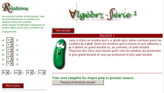
|
|
|
|
|
Fig. 4: Example of feedback given for the trials of one student (task in series-1) |
||
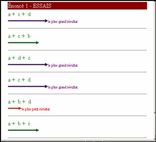
After students have completed all the tasks for series 1 and 2, they are given a quiz. Below are some of the questions of that quiz. We show some of the answers given by students. The students were invited to choose between
a) ?
b) AT : always true
c) ST : sometimes true
d) AF : always false
e) SF : sometimes false
They also have to justify their choice. As we can see in Table 2, the justifications of the students of class A were generally explicit.
Table 2: Answers of students to some of the questions in the quiz on natural numbers
|
Questions |
? |
AT |
ST |
AF |
SF |
Justifications |
|
p + a + z + z = |
|
|
Eq-1,3,7 |
Eq :2,4,5,6 |
|
Eq :1,2,3,7 : z = 0 Eq-4 : we add two numbers and one Eq-5 : we have 4 numbers and 3 numbers |
|
px (a + b) = (px a) + b |
Eq :4,5,7 |
Eq-6 |
Eq-3 |
Eq :1,2 |
|
Eq-1 : we multiply two numbers added Eq –2 : we have to multiply by b Eq-3 : suppose b = 0 Eq-4 : with parenthesis Eq-5 : with () priority |
6 Conclusion
Preliminary results from our study show significant increase in learning among students who have participated in experiments done with the two computer environments. The conjunction of both environments seems pertinent; students had the opportunity to “decontextualize” knowledge used in previous calculation tasks. The ease with which they entered into the third environment was probably due to the fundamental work done in the second environment. It should be remembered that these students had no previous experience with algebra.
Concluding remark
The environments we have built are still being submitted to validation and transformation. The results obtained so far are significant. These environments were also received with enthusiasm by all the teachers who were involved in our experiments.
References
Brousseau, G. (1998) Théorie des situations didactiques, [Textes rassemblés et préparés par N. Balacheff, M. Cooper, R. Sutherland, V. Warfield]. La pensée sauvage, coll. Recherches en didactique des mathématiques, Grenoble.
Chevallard, Y. (1985) Le Passage de l’Arithmétique à l’Algèbre dans l’Enseignement des Mathématiques au Collège. Petit x, 5, 51-94.
Chevallard, Y. (1989) Le Passage de l’Arithmétique à l’Algèbre dans l’Enseignement des Mathématiques au Collège. Deuxième Partie: Perspectives Circulaires: la Notion de Modélisation. Petit x, 19, 43-72.
Combier, G., Guillaume, J.C. et Pressiat, A. (1996) Les débuts de l’algèbre au collège : Au pied de la lettre! INRP, Paris.
Devauchelle, B. (1999) Multimédiatiser l’École? (Série dirigée par J.- P. Obin). Hachette Education, Paris.
Julo, J. (1995). Représentation des problèmes et réussite en mathématiques : un apport de la psychologie cognitive à l' enseignement. Presses Universitaires de Rennes, Rennes.
Acknowledgement
This project was subsidized by FCAR-Québec et CRSH-Canada. We wish to thank all the teachers and students who have generously contributed to the success of this project. We also wish to thank Félix Famelart who has assumed a good part of the English version of the French paper.
To learn from and make history of maths
with the help of ICT
Marie-Thérèse Loeman
Sint-Niklaas, Belgium
1. Start and (initial) objectives
2. Motivation for the teachers to put extra effort and time into this project
The report below gives results from the EEP Comenius Action 1: "The history of some aspects of mathematics like : history of mathematical persons, symbols, algorithms…":
http://mathsforeurope.digibel.org/
1 Start and (initial) objectives
The idea was conceived during the European Comenius Contact Seminar " Europe, you can count on it! " held in Antwerp (BE), June 1997 where teachers from the three initial upper secondary partner schools from Sint-Niklaas (Belgium), Vittorio Veneto (Italy) and Greåker (Norway) met for the first time.. The plans of the project were approved by the three national agencies in March 1998. During the second project year a new partner school of Mikkeli (Finland) joined the group.
The aim of this project work was to encourage our students -during the lessons as well as on a free basis, e.g. with an extra home work of maths, history, and philosophy- to investigate on the one hand the existence of important mathematicians who lived in the participating countries and on the other hand the origin and the development of mathematical symbols, algorithms...
In addition we wanted to make use of the new ICT (Internet + e-mail) and involve an intensive exchange of information and experience on innovative methods of teaching. This exchange, giving also the opportunity to learn from the stronger elements in each partner country, would be best served by using the English language (being taught in all partner schools). The teachers of maths, history,… in each country would try to incorporate in their lessons the gathered results and publish them on the net.
Taking into account the cultural and traditional background of each partner and the different stage of development of ICT in each country, we wanted to allow each school to develop one or more aspects of maths completely or in part at their choice.
2 Motivation for the teachers to put extra effort and time into this project
Starting from the belief that teaching maths should not be reduced to practising rules, the project wanted to
stimulate
the love for maths and creative thinking
encourage
students to look at the problems from a wider point of view, in a
multidisciplinary context, making links to other fields like philosophy
make
students learn from the great thinkers of the past and present
This
last is because we want the students to be aware of the fact that concepts found
by ancient, modern and contemporary mathematicians served and will serve our
present and future society.
Practical arrangements for the project work
Presenting the project to students aged 16 to19, we allowed them to choose a topic related to maths, which particularly attracted them. We encouraged them to work in groups, to divide tasks between them and look for information in books and on the net. The work they were going to put together should present material, which they could understand with their own mathematical background. At best, the work should also contain some special (historical) detail or pictures, which would encourage future readers to keep on concentrating. According to their ability, with the help of engaged teachers and enthusiastic parents, they could hand in their results on a disk or send it by e-mail to the coordinator or put it themselves on the net using Frontpage.
3 What did we get?
At first of course some small biographies of mathematicians
Our students and teachers involved became more and more convinced that it is not only the results found by great mathematicians that are important for us. Getting to know the ways they thought and found the solution to the problems that puzzled them (considering the means available at their time in the historical context they were living in) is also very instructive and sometimes even inspiring. Often students have a fixed (wrong) idea about maths (too hard for me, too boring, old-fashioned...). From the historical notes they observed that great mathematicians also had to surmount many obstacles (e.g. Euler being blind for some years and still very productive). These great thinkers were not always the best performing students in the learning system that was available to them at their time. Moreover, being a mathematician, they often had to face and struggle against constant opposition even from some of their colleagues, and also from society and the religious environment (e.g. Galileo). But despite that, they all could not resist thinking and searching for the solution and explanation (proof) of the item they were investigating. Nowadays students can check for themselves, e.g. with the graphical calculator, the laws Galileo Galilei defended.
|
|
|
|
|
|
|
|
|
|
|
|
Fig. 1 |
|
|
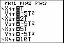
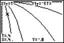
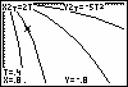
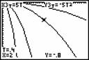
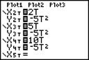
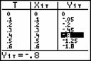
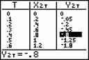
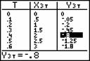
Looking through the different biographies, the students also became convinced that the history and development of maths has always been related to other scientific subjects like physics, astronomy, geography, construction, economics… A lot of famous mathematicians were at the same time engineers! Developments in maths often originated from what could be used in a situation where a solution was urgent in their society (Archimedes, …).
In our times, apart from pure maths thinkers, experts in applied mathematics are again in great demand. On the other hand we do not live by bread alone. We also need games (Probability), beauty (Golden Section) and magic (Magic Squares). Important principles were found going deeper into what was first considered as a luxury e.g. exploration of the universe (the development of computers), the internet, philosophy… the latter having had a great impact on the development of the conditions of human life.
Study of some special topics
they had met before although not in maths lessons: for instance the designs of Escher, Fractals, The Golden Section.
|
|
|
|
|
Fig. 2 |
Fig. 3 |
Fig. 4 |

Study of the number systems in different cultures
(Egyptian, Greek, Roman, Maya, Indian). Students found out that from the beginning, and in different civilizations, symbols and a base were chosen for their number system. What base was chosen (2 or 20 or 10 or …) was related to e.g. economical activities or even their calendar (e.g. the Maya calendar which happened to be very accurate). We discussed in the lessons that for practical reasons the decimal counting got the leading banner in sciences and maths, but the binary system used in the development of calculating machines and computers, was already known by the Egyptians. In the following figure, parts are taken out of the project works Egyptian maths and the pyramids, Simon Stevin, Maya numerals.
|
|
|
|
|
|
Fig. 5 |
|
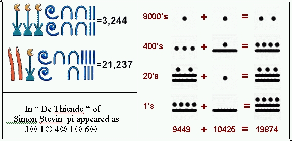
We were amazed to see how the notation (pictorial or …) of the numbers was related to a culture and showed some evolution, as the numbers were used to make calculations and at a later stage to solve equations. After some time notations became positional, taking in account the base, written from left to right, and higher to lower order (apart from the Maya system which was also sometimes written from top to bottom). All of them had, as we still do, some special meaning (bad luck or… ) to certain numbers (see the work of Numerology). Knowledge of the existence of special numbers like pi and e also grasped the attention of some students.
Even when several groups in different countries made a contribution to the same topic, we discovered underneath their different interests. (In the work on Egyptian maths and pyramids, the leading student had a great devotion for science fiction which can be noticed from the part comparing the construction properties of the pyramids with the constellations of craters on the planet Mars). The more they gained insight into the different topics through history (Fibonacci sequence, golden section, fractals and even chaos) the more they become aware that all these parts come together in a greater whole.
We encouraged students’ own creativity
We encouraged the students also to try out something on their own initiative, and using their own creativity, (for instance, in the work on Magic Squares, colouring the multiples of two, etc, in different colours getting fascinating patterns;
|
|
|
|
|
|
Fig. 6 |
|
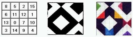
and in the work on Polar Math Art getting different ‘flower’ curves)
|
|
|
|
Fig. 7 |
Fig. 8 |
|
R = (1.5) ( 1-abs (-sin (6(t-1)))+ 2(cos(2(t-1)))) R = (1.5) ( 1-abs (-sin (6(t-1)))+ 2(cos(2(t-1)))) - 0.5 R = (1.5) ( 1-abs (-sin (6(t-1)))+ 2(cos(2(t-1)))) – 1 R = (1.5) ( 1-abs (-sin (6(t-1)))+ 2(cos(2(t-1)))) - 1.5 R = (1.5) ( 1-abs (-sin (6(t-1)))+ 2(cos(2(t-1)))) –2 |
R = (3.5)(3-abs(sin (4(3t-1)))+ 4(cos(2(4t-5)))) R = (4.5)(3-abs(sin (4(3t-1)))+ 4(cos(2(4t-5)))) R = (5.5)(3-abs(sin (4(3t-1)))+ 4(cos(2(4t-5)))) |
Working together with students of partner schools
During the 3rd year of the project we wanted the students of all partner schools to work at the same time on the same topic. The repeated The experiment of Eratosthenes (needing their trigonometry and geography lessons), and they reflected on the results of the expedition of Maupertuis and the triangulation method. This was also the start for another maths investigation about The hours of daylight (mostly regarded as a normal sine curve which is certainly not the case the closer we get to the polar circle). They felt the need to ask for information from university professors and the astronomical observatory in the different countries.
Gaining the attention of the students
We also gained the attention of our Scandinavian friends with a much-appreciated product like beer and liquor (work of Duvel, Trappist, Volume of drinking glasses etc). Even low achieving students in maths could be motivated to use their knowledge of integral calculus and the regression features of the calculator to calculate the volume (inside) of some beer or other glasses. It is interesting to notice the different approaches of performing the physical measurements.
|
X Y 0 0 0.5 2.1 1 3.4 1.5 4.2 2 4.8 2.5 5.0 3 5.1 3.5 5.0 4 4.8 4.5 4.5 5 4.3 5.5 4.1 6 4.1 6.5 4.0 7 4.1 7.5 4.2 8 4.2 [in cm] |
|
|
|
|
|
|
|
Fig. 9 The thickness of the glass and of the pencil were taken in account! |
||
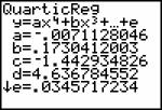
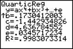
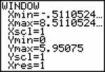
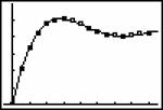
Connecting to classical architecture
Because of the Italian liceo involved in the project (which could provide interesting material) and the input from our Flemish classes (where classical Greek and Latin is still a main subject), we could encourage the students to investigate the Maths behind the beautiful, almost acoustically perfect, and solid constructions of old theatres and amphitheatres. The Cabri programme was used to illustrate the way sound rays are sent throughout and kept inside the elliptical arenas in optimal conditions.
|
|
|
|
|
Fig. 10 |
Fig. 11 |
Fig. 12 |
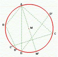
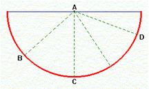
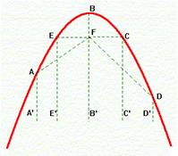
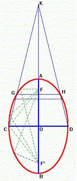
All Roman amphitheatres are elliptical because the ellipse is the ideal figure to guarantee the best distribution and amplification of sound throughout the theatre. If the centre of the transmission lies on the circumference of a circle, we observe that all sound rays are reflected in different directions. If the sound has its origin in the middle of a semi-circle, each ray is reflected back to the origin. Starting from the focus of a parabola, all waves disappear parallel to the main axis. But if the sound emerges from one of the foci of an ellipse then, from mathematics, we know that all waves will come together in the other focus. As a result a second centre of sound is created that will amplify the original sound. In addition the Romans kept the golden ratio (phi) as the uniform proportion in their construction (main axis/small axis of the basic ellipse, width/height of steps, width/height of the rows around the arena…).
Conforming to the ideas of Vitruvius, in order to get a good view and reception of the sound at each point in the theatre, the maximum angle of inclination should not exceed arctan (1/phi) and the largest distance from the nearest focus |KF| should be smaller than or equal to |BF|. Once the axial dimensions of the basic ellipse shape of the plan were decided, the same module of load-bearing walls containing the staircases and surmounted by barrel- vaulting had simply to be replicated a certain number of times until they joined.
Apart from trying to achieve a solid construction and aesthetic harmony, for the thoroughly practical and realistic Romans the decision to work to proportional measurements made it possible to have the work done by several groups, not necessarily supervised by a single architect but rather by a team, and still ensuring effective coordination of all building operations.
The interaction politics versus maths
also became clearer, reading that great mathematicians were helped by some mecenas; kings and governors who sponsored many scientists for strategical reasons. An illustrious example is Napoleon who, although being himself a mathematician !?!, surrounded himself by Laplace, Monge, Fourrier, Lagrange..). Nowadays sponsoring is often done by the new rulers of the world (e.g. powerful companies). And always, the work of mathematicians (Einstein) can have a considerable impact on achieving peace and a better life on our planet.
4 Effect on our teaching
Stimulating the students to do some work for the project has also some consequences for our way of teaching: instead of making students do several drill exercises and having them memorize many similar proofs, we prefer to present them with different patterns and special ways of thinking (e.g. the reasoning of Euclid to prove that the sequence of primes is infinite). In solving a problem, not only is the solution appreciated but also a nice, perhaps different and preferably original way of finding and proving it. This is what makes the scientist superior to the machine!
In most countries the school systems provide a heavily loaded maths curriculum (certainly more than in e.g.. the time of Newton because of the growing amount of important discoveries) so doing all the calculations and constructions over again ‘by hand’ leaves no time nor occasion to try out different thinking patterns…Having such a great amount of interesting maths topics to teach the students, we ‘must’ let them use, as much as they can and wish to, the facilities of the calculator, the computer and computer programmes, the internet and other new communication technologies, in order to make time and opportunity and space to do some ‘creative’ thinking. Besides the continuous passing through of information and of discoveries already found and proved, encouragement of this thinking is crucial because the machines will always need to be programmed accurately.
Digging in the history of maths and working together across subjects (also co-operating with colleagues who are teaching other subjects like English, religion, philosophy, chemistry, geography, physics, music…) is also a source of inspiration. Teachers get more ideas for questions for tests and examinations. As an example, we used the problem on triangulation (see work of Mercator), explained by Gemma Frisius in his book Libellus de locorum describendonum ratione (1533), in our tests in trigonometry. Mercator was born in the neighbourhood of Sint-Niklaas, which is the town where the Belgian partner school is located and where the drawing and the text of Gemma Frisius hang on the wall in the Mercator museum.
“One starts drawing a circle with a meridian (the diameter) on two different pieces of paper. Afterwards he climbs on the tower in Antwerp and puts one circle in the right position (the meridian north-south) using the compass needle. He draws lines in the direction of the adjacent cities: Middelburg, Gent, Brussel, ....taking that tower in Antwerp as the centre of the circle. With the circle on that other piece of paper he repeats the procedure looking out from a suitable tower spire in Brussels towards the other cities. Coming home he puts the two papers at an arbitrary distance from each other but keeping the two meridians parallel. Prolonging the lines of the different directions (which he drew at the top of the towers) he gets the exact location of the cities at the points of intersection. Starting from the distance between Antwerp and Mechelen (four units), dividing this segment in four and comparing with the other segments, one can find all the distances between the different cities on the map.”
The drawing to the left is hanging in the museum and the drawing to the right was given to the students. Given that½AM½= 4 units, ÐGAD = 83°12’, ÐDAM = 24°, ÐABC = 26°50’, ÐCBG = 58°15’ and ÐMBC = 60° they had to calculate the distance from G to M (applying the sine and cosine rules and using small programs the students made and put themselves into the memory of their TI-83 calculators).
|
|
|
|
Fig. 13a |
Fig. 13b |
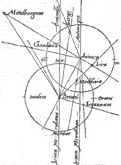
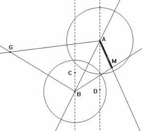
Because this work is staying on the net for the time being (given free of charge), the information found can be used in lessons for other or future student groups.
5 Effect on the students
Considering that maths is only one of many subjects in the school system, it is most likely the students will not remember all the series of calculations and proofs we presented them with. But letting them investigate for themselves how other young minds before them explored, using all possible tools, different ways of mathematical thinking and the use of this thinking, will help them forever and will certainly last longer. Even students with less interest and lower achievement in maths were interested in some part of the project: e.g. making the design for the cover of the CD (for educational purposes a copy of the CD can be obtained from the coordinator: mth.loeman@pandora.be) improved their opinion about our so-called ‘hard’ subject .
Looking through the topics in co-operation with students from other nationalities and cultures convinced them that maths, because of its special common language and symbolic notations, has no boundaries. In addition they became more appreciative of and were encouraged to learn from the stronger elements in each partner country: teaching and use of ICT in Norway and Finland, philosophical thinking and search for proportion and beauty in Italy, believing in the strength of a unified system and intensive (team) work in Belgium. Also finding out that they have the privilege to be taught by inspired teachers (mathematicians from the past and the present) will improve their willingness to make some effort (studying, working carefully and with great effort to investigate a clear and solid solution for some problems) to be able to discover the magic and power (still leaving opportunities for more discoveries and explorations) of our special common passion: mathematics.
Acknowledgements
to all the maths teachers who ‘inspired’ my interest for maths and teaching maths: among them certainly the late Prof. Roger Holvoet (University of Louvain/BE) and Prof. George Polya (Stanford University/California-USA), and to the European Commission and the Norwegian Socrates Agency (SIU) and all the private companies, mentioned on the project website, who sponsored the project.
Thinking the unthinkable —
Understanding 4 dimensions
Proposal for a training course in four-dimensional perception
Claus Meyer-Bothling
Stuttgart, Germany
1. The world is at least 4-dimensional
2. Characteristics of 4-dimensional bodies
3. What does this mean for us?
If you mention the fourth dimension, people tend to think that you are prone to irrelevant speculations or that you are a science fiction author. However, if we take account of what is possible today, with the latest technology, this might soon change. After following the training course that I am presenting in this paper, soon all of us may be able to perceive 4-dimensional objects directly.
1 The world is at least 4-dimensional
First of all we have to realise that the 4th dimension is not theoretical. It is a practical fact, which follows from Einstein’s General Theory of Relativity. In order to avoid misunderstandings here: I do not mean 4-dimensional space-time, but I am actually talking of the 4th spatial dimension. (If we included time as well, we would obtain 5-dimensional space-time. However, we do not have to consider time in this context, because we are not concerned with high velocities.)
|
The central statement of the General Theory of Relativity is that space is curved by the presence of mass. In popular representations the curvature of space is usually symbolized by funnels that somehow hover in space, but this only distracts from the actual problem: our imagination is massively overtaxed. Space curvature – how on earth are we to imagine that? |
|
|
Fig. 1: Funnels symbolize curvature of space (Karamanolis 1987) |
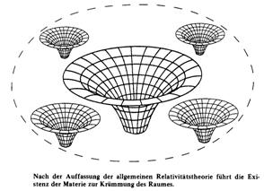
A comparison might serve to illustrate the problem: we can certainly envisage bending a 1-dimensional straight line and we can demonstrate this by bending a straight wire. It becomes apparent that for bending the 1-dimensional space at least one further linear independent direction is necessary, i.e. at least one further dimension. If we remained within the one dimension of the wire, we might be able to stretch it - bending would not be possible. Similarly we can bend a flat 2-dimensional space, represented by a flat piece of paper, only if a third dimension is available. And finally, in order to bend a 3-dimensional space of course we require a 4th dimension.
Let us for a moment imagine a society of 2-dimensional beings, which are conscious of only 2 dimensions. Let us further imagine that these „flatlanders“ live on the surface of a large sphere. Can they know this? If they are mathematically trained, they can measure that the sum of the interior angles of large triangles clearly exceeds the 180°, which would be expected in a flat Euclidean space. They would have to conclude that their 2-dimensional space is not flat, but curved. From that they could deduce that their perceived 2-dimensional world is embedded in a reality of at least 3 dimensions. This does not imply that they can really imagine the 3rd dimension, but they would at any rate have proved its existence.
We ourselves are in an analogous situation: the space that we can habitually imagine has 3 dimensions. As we are sure that it is curved, we are also certain that our perceived 3-d-space is embedded in a reality of at least 4 dimensions.
2 Characteristics of 4-dimensional bodies
The characteristics of 4-dimensional bodies, such as a 4-d-cube are well known in mathematics, although – following the popular view – this has no relevance for real life. We can even understand a 4-d-cube, if we take a look at „cubes” in up to 3 dimensions. We can produce a cube of dimension n by shifting a cube of dimension n‑1 toward a new dimension. With the usual designations we arrive at this line-up:
|
Dim. number n |
0 |
1 |
2 |
3 |
4 |
|
name |
point |
line |
square |
cube |
tesserakt |
|
object |
|
|
|
|
|
|
Fig. 2 |
|||||


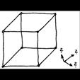
Of course we have difficulties imagining in which direction to shift the 3-d-cube, in order to obtain a hyper-cube or tesserakt. Nevertheless further characteristics of the tesserakt can be understood by analogy.
|
Corner points |
1 |
2 |
4 |
8 |
16 |
|
Delimitations of dimension (n-1) |
- |
2 points |
4 lines |
6 squares |
8 cubes |
Still our imagination fails with the tesserakt: how are we to envisage a figure with 16 corner points and 8 delimitation cubes?
In this situation it helps that the geometrical shape of the tesserakt can easily be determined by calculating its corner points. Let us imagine that the origin of the coordinate system is situated in a corner point of the figure, that the side is chosen as unit, and that the figure extends into the positive region of the coordinate system. The coordinates of all corner points can now be determined by writing down all combinations of the coordinates 1 and 0. This works for any number of dimensions:
|
Coordinates of the corner points |
- |
1 0 |
(1;1) (1;0) (0;1) (0;0) |
(1;1;1) (1;1;0) (1;0;1) (1;0;0) (0;1;1) (0;1;0) (0;0;1) (0;0;0) |
(1;1;1;1) (1;1;1;0) (1;1;0;1) (1;1;0;0) (1;0;1;1) (1;0;1;0) (1;0;0;1) (1;0;0;0) |
(0;1;1;1) (0;1;1;0) (0;1;0;1) (0;1;0;0) (0;0;1;1) (0;0;1;0) (0;0;0;1) (0;0;0;0) |
Up to the 3 dimensional cube this can be confirmed from direct perception. Still we cannot imagine the 4-dimensional tesserakt, but it is now determined through its corner points. It can be plotted in a virtual 4-dimensional space. If we subsequently project it onto our habitual 3-d-space, we can build a wire model of the tesserakt. This in turn can be sketched on a piece of paper. For the fourth direction we use the same trick that we know from drawing the 2-d-representation of a cube: we simply choose a new direction in the lower-order space.
|
|
|
|
Fig. 3: Sketch of the cube |
Fig. 4 Sketch of the tesserakt |
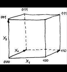
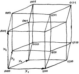
Other elementary 4-dimensional bodies, e.g. the sphere, can be determined similarly. From the elementary bodies, more complex bodies can be developed. If the lengths of the sides of a tesserakt are made different, we obtain the more general 4-dimensional cuboid, which is delimited by eight 3-d-cuboids. If we omit one of these, we obtain the 4-d-equivalent of an open rectangular box.
3 What does this mean for us?
We know that reality is at least 4-dimensional. Through mathematics we also know a great deal about the 4th dimension. Still, we cannot imagine it. Although we do have rational access to 4th dimension, it is non-existent for our senses and for our consciousness.
Obviously there is a whole dimension that escapes our perception.
Two questions arise from this: how is this possible, and what can we do to change it?
How is it possible that we are missing a whole dimension?
Two factors seem to be responsible. Firstly the space curvature in our environment is relatively small. Einstein (1988) commented on this:
Es ist .. denkbar, dass unsere Welt von einer euklidischen [nur] wenig abweicht, diese Auffassung liegt umso näher, als die Rechnung ergibt, dass selbst Massen von der Größe unserer Sonne die Metrik des umgebenden Raumes nur ganz minimal beeinflussen. Man könnte sich vorstellen, dass sich unsere Welt in geometrischer Hinsicht analog verhält einer im einzelnen unregelmäßig gekrümmten Fläche, die aber nirgends bedeutend von einer Ebene abweicht, wie etwa die durch schwache Wellen gekräuselte Oberfläche eines Sees.
Secondly, the perception of our environment has developed in the course of millions of years according to Darwin’s principles of variation and selection. I.e. it is based not on correctness and completeness, but on appropriateness in the struggle for survival. In other words, our perception is not true, but useful. If our environment has not much of a structure in the 4th dimension, perceiving the 4th dimension possibly does not yield enough advantage to make it worthwhile in the struggle for survival. Nonetheless it remains unsatisfactory that a whole dimension escapes our perception.
What can we do?
Although people have tried in vain for over 100 years to close this gap in our imaginative power, we are now in a better position than all our predecessors. The difference is due to new technology available today and research into the way perception works. In order to explain, I shall first report on 3-d-perception, and subsequently apply the observations to 4-d-perception.
4 3-d-perception
Formation of 3-d-perception with children
The perception of spatial depth begins in early childhood, but takes many years up to its full development. Piaget differentiates the following phases (Piaget and Inhelder 1975):
|
|
Phases of perception |
Order criteria |
Beginning |
|
I |
sensory spaces (seeing and feeling) not coordinated |
Proximity, separation, sequence, being enclosed |
|
|
II |
Coordination of seeing and feeling |
Figure, constant perspective of form and size |
4-5 months |
|
III |
active experiments, from perceived to imagined space |
relation between objects |
2 years |
The crucial phase in the perception of spatial depth begins, when the baby goes beyond mere optical perception and starts to actively intervene through groping and feeling. We might think of typical behaviour in early childhood, where the baby lies on its back, seeing but also touching, using its arms and legs to explore the environment, thus coordinating the separate channels of perception. Through this coordinated exploration the child relatively soon develops a conception of spatial depth, the 3rd dimension, which becomes more differentiated over the years.
|
|
|
|
|
Fig. 5: Baby, tentatively exploring its close environment |
||

The gradual development of spatial depth can be observed very beautifully, in comparing children’s drawings at different ages.
|
|
|
Fig. 6: Children’s drawings, age 7, 6, 9, 11, 13; from Kerschensteiner (1905) |


Although these drawings document stages of representation rather than perception, they can give us a good impression, that the consciousness of the spatial arrangement, both laterally and in depth, is being differentiated over the years.
For the development of our consciousness of the world we have several channels of different quality at our disposal. The optical channel supplies us with information at high resolution if at first only 2-dimensional. Active groping and feeling are of inferior resolution, but supply information on the depth structure of space. Our consciousness learns to combine fragments from different channels into an overall view, which is of a higher dimension, or better resolved, than the information from each individual channel. Apparently it is 3-d-action, which finally raises our perception and our consciousness from 2 to 3 dimensions.
Perception with adults
Objective perception?
Common sense, on which we largely rely in everyday life quite naturally and successfully, does not allow any doubt that we perceive the environment as it really is. This naive conception, that we perceive the environment objectively, is also supported by the simplified picture of optical perception, which seems so plausible: the eye projects an objective picture of the environment on the retina, just like a camera. The retina registers this picture and the brain stores it, just like the CCD and RAM in a digital camera.
3-D-perception happens through many channels
According to the naive view our retina image is no more than a 2-d-reduction of 3-d-reality. However with increased practice we do use a number of additional optical signals, that we learn to decode involuntarily (Gibson 1973):
Geometrical
perspective - 2 eyes with 2 different lines of sight
Comparison
of size - near bodies are larger than distant bodies
Concealing
- near bodies cover distant bodies
Luftperspektive
- “air perspective”, colours fade in the distance
|
|
|
|||
|
Fig. 7: Coastal landscape in the morning and in the evening: on the right the Luftperspektive supplies us with additional information about spatial depth. |
||||


Obviously perception is not a pure process of registration but it is already strongly coupled with interpretation. This makes adults’ perception, strengthened by experience, so efficient. The trained 3-d-consciousness can even construct a 3-d-world on the basis of reduced information: even with one eye closed we can walk through our own house, or even unknown environments, without running against furniture or walls.
Colour hallucinations
|
The naive view of objective perception must be differentiated even further on the basis of this experiment: Blow the image of the light bulb up and look at it for a few minutes. Then look at a white background. Our perception, developed in the struggle for survival is not optimised for objective rendition of colour and brightness, but for optimal detection of modifications and differences. Thus a constant perception of colour or brightness is more and more assumed as neutral background. Subsequent observations are then interpreted on this basis. |
|
|
Fig. 8 |
Space interpretations
|
In some cases the interpretation goes so far that it even becomes an obstacle to objective perception (impossible object). The quick 3-d-interpretation of optical impressions, which helps us so much in daily life, here stands in the way of objective perception. Really, this is not a picture of a spatial arrangement, but a refined trap for our brain’s involuntary interpretation process. |
|
|
Fig. 9: Interpreted as triangle - an impossible object |
Efficiency of adults’ 3-d-perception
The above examples show that our perception works very efficiently. It does not merely supply us with an objective image of the environment, as it really is, but it applies various processes of filtering and interpretation that have proved helpful over the millions of years in the struggle for survival as the basis for fast decisions (attack, flee, or try to make friends).
We can now apply this observation to the 4th dimension. The fact that we cannot habitually perceive it does not mean that it does not exist, but rather that perceiving it would not have helped sufficiently in the struggle for survival to justify the effort.
However, today we can dispose of methods of changing the environment convincingly in order to make it worthwhile for our perceptive apparatus to perceive 4 dimensions. Nevertheless, the ability to perceive 4-dimensions after many years of 3-d-perception sets high demands on the adaptability of our perception. Yet there are experiments that show impressively how adaptable our perception apparatus really is.
Adaptability of our perception
|
Since 1896 there have been investigations into how the visual perception of adults changes, when it is disturbed, and after the disturbance has stopped. The first experiments took place in the laboratory. Test subjects wore prism eyeglasses which distorted and laterally shifted their visual field. As expected the subjects at first had great difficulties in their orientation. Surprisingly though, after just a few days the subjects got used to their distorted vision. After the eyeglasses were removed again, a shorter habituation time was necessary, until the subjects could orient themselves normally again. |
|
|
Fig. 10: Die Umkehrbrille (Erismann-Kundratzitz) |
In 1928 Erismann began a spectacular series of investigations in Innsbruck (Kohler 1951). He did not merely shift the field of vision, he inverted it - i.e. the subjects’ field of vision was turned upside down. In an improved series in 1947, the subjects wore specially designed mirror eyeglasses, which not only inverted the visual field, but were even inconspicuous, because they could be hidden under a peaked cap. With these the subjects, all volunteers, could continue wearing their reversal eyeglasses in their normal life without provoking much attention. Some of the experiments were continued over 50 days.
|
A relatively short experiment of only 6 days is commented on like this: Die Vp. sah in den ersten Tagen durch diese Brille alles verkehrt, von unten nach oben hängend, machte ständig Greiffehler, war höchst unsicher, mußte begleitet werden. Nach drei Tagen erstaunliche Besserung des Verhaltens, am vierten eine Fahrradtour, am letzten sogar ein kleiner Skiausflug. The experiment shows typical elements: for the first few days orientation was difficult. Within a short time reorientation occurred. After that the test subject again had a correct and increasingly stable consciousness of the environment, which permitted even relatively fast reactions like in a ski excursion on the 6th day of the test. |
|
|
Fig. 11: Regaining stable consciousness |
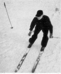
Another subject continued wearing the reversal eyeglasses for over 50 days. Towards the end he could even wear them driving a motorcycle - not over a quiet dirt road, but through the city of Innsbruck. No accident was mentioned in the report.
|
We ourselves, not having taken part in these tests, can hardly imagine that someone can see the world upside down and still move safely in it. But that is not what really happened. During the reorientation the subjects adapt to the new vision and in fact see the world upright again. We have to imagine a mental flipping over that happens in the consciousness of the subject, much like what happens, when you see the set of stairs in two different ways (Umklappfigur). |
|
|
Fig. 12 |
Our tremendously efficient perception apparatus apparently adjusts to a new optical view, using the same methods as in early childhood: the combination of seeing and feeling leads to the re-orientation of our perception apparatus. Additional exercise serves to stabilise the new adapted mode of perception until you can even drive a motorcycle with it.
2-d-seeing, as well as 3-d-action result in a newly-oriented 3-d-consciousness, which is strong and reliable again.
5 4-d-perception
This can now be applied to the perception of the 4-d-reality. If we manage to increase the two major channels by 1 dimension each, thus achieving 3-d-perception and 4-d-action, we could successfully develop a 4-d-consciousness of the world.
New technology
|
|
Seeing |
Feeling |
Consciousness |
|
Infants |
2D |
3D |
3D |
|
Adults in a virtual world |
3D |
4D |
4D |
Today, owing to new technology, this seems feasible: Virtual 3-d environments with 3-d-action have already been in use for some years. They are being used in industry, e.g. for the development of new car types at Daimler-Chrysler. The Fraunhofer Gesellschaft has recently presented a new efficient and relatively cheap system, their “6-Side-Cave”. 4-d- worlds can easily be developed in virtuality. Force-Feedback may yet be some way off, but is not necessarily required.
Organization of the training course
The virtual environment is modified in such a way that actions are possible not only in three but in 4 dimensions. The control signals for motion in the conventional three directions in space can be given as usual. A further parameter will have to be dedicated to motion in the 4th direction. Thus the test subject can move an object in 4 dimensions. The software calculates the resulting modifications of the 4-d-objects, and represents them in their projection in 3-dimensions. The subject is thus in the same position which is mastered by each infant one dimension further down.
We begin with simple 4-d-objects, such as cubes, and cuboids. Suitable transactions are displacements and rotations. The first tasks are of the type: „Put the cuboid into the box. Remove it again and put it down on the right beside it. Rotate it so that it goes in into the small box.” Test subjects are volunteers who have passed a test assessing their spatial imagination.
6 Reality in 4 dimensions
Much has already been written on the 4th dimension and we have to distinguish carefully between knowledge and speculation in order not to be misunderstood. However, one thing is certain: If we could master 4 dimensions in the same way as the habitual 3, our life would have to change radically. It would not be possible e.g., to keep objects in a box or in a room safe from foreign access. A being operating in 4 dimensions would still have free access to the objects. An extensive and lucid compilation of similar qualities of the 4-dimensional world offers Rudy Rucker (1984)
Then again we have to distinguish between perception of the 4-dimensional world and operating freely in 4 dimensions. A training course of the type suggested here only influences perception, so that possibly our life would not have to change quite as radically as I have just indicated. Even so, a being with unrestricted 4d-perception could look into closed rooms...
In this context there are many open questions, and there has been speculation on the answers for a long time. My suggestion follows our western scientific tradition: let us make an experiment! In the past the experiment has not been possible, only now we are in the thrilling position that we can decide on the theoretical questions through practical experience. It would be unthinkable for me, not to take this chance.
How the project proceeds
The project is in the planning stage. Principal partner for the implementation is the Fraunhofer-Gesellschaft.
Trial
All phases of the experiment will be gone through. Test persons are the members of the scientific team. Different exercises will be developed and informally tested. Duration: 6 months. Cost: € 45,000.
Main experiment
If the trial ends with encouraging results: refinement of the experiment in line with psychological and statistical requirements. Implementation of the refined experiment under defined conditions. Duration: 12 months.
Results of the project
If the subjects succeed in imagining or perceiving 4-d-reality directly, this would be a tremendous success as well as the foundation for a new area of research
If the subjects do not succeed in imagining 4-d-reality directly, the experiment has still brought forward a question that provokes further research: why can we not perceive the 4th dimension, even so it exists?
At any rate techniques will be developed in the course of the experiment to represent multidimensional relations in a comprehensible way. These can easily be transferred to other areas of science and technology.
A further area of application is didactics. If we apply the methods developed during the project on 3-dimensional bodies, i.e. on a regular subject taught at schools and universities, we can teach Geometry in virtual space. Students can thus experience interactively any geometrical structure. This would constitute a considerable extension of the possibilities in use to date.
References
Einstein, Albert (1988) Über die spezielle und die allgemeine Relativitätstheorie. Braunschweig.
Erismann, Theodor (1962) Allgemeine Psychologie III. Berlin.
Gibson, James J. (1973) Die Wahrnehmung der visuellen Welt. Übers. Vera Schumann. Beltz, Weinheim.
Karamanolis, Stratis (1987) Einstein für Genießer. München.
Kerschensteiner, Georg (1905) Die Entwickelung der zeichnerischen Begabung. München.
Kohler, Ivo (1951) Über Aufbau und Wandlungen der Wahrnehmungswelt. Sitzungsberichte der Österreichischen Akademie der Wissenschaften 227 Band 1.
Piaget, Jean and Inhelder, Bärbel (1975) Die Entwicklung des räumlichen Denkens beim Kinde. Stuttgart.
Rucker, Rudy (1984) Die Wunderwelt der Vierten Dimension. Scherz, München.
Up to date information on the project: www.zum.de/faecher/a/bw/4d
Remedial education of quadratic functions
using a web-based on-line exercise system
Hitoshi Nishizawa, Yasuto Kajiwara, and Takayoshi Yoshioka
Toyota, Japan
2. Expressing a quadratic function symbolically
3. Students’ ways of expressing quadratic functions
5. Remedial education using the on-line exercise system
6. Effectiveness of the on-line exercises
The method and the effectiveness of remedial education using a www-based on-line exercise system are reported in this paper. The system displays graphs of quadratic functions on the students’ screens and requests them to express them symbolically. Six students, who had difficulty in this type of exercises with pencil-and-paper, were selected to attend the remedial course using the system. Although their symbolic expressions had depended upon quite limited formulae before the on-line exercises, they extended the variety of their expressions through the remedial course. The learning was effective when the quick response of the system and the peer help were combined together. The on-line exercise system was found to be a good supporting tool of remedial educations.
1 Introduction
Graphic and symbolic representations of a mathematical function compensate each other in a human mind when it tries to use the knowledge of algebra to solve a problem in the real world. A symbolic representation helps to build a mathematical model for the problem and solve it. A graphical representation is suited to investigate the solution and interprets it to the real world. Detailed investigation of a graph requires the exact knowledge of the relation between the graph and the symbolic expression.
For constructing the knowledge, the uses of CAS or DGS have advantages. Exploration supported by technology attracts students, provides them with the experience of trials and errors, and helps to find the common rules there. It would be a good way to teach mathematical literacy for the users of mathematics (Fukuda 2000).
For advanced users of mathematics like engineers, deeper understanding of mathematical functions is required. They are expected to know the detailed relation between a symbolic expression and the graph. They should learn the mechanism to connect two representations together as their own knowledge. Because the technology generally does not explain the intermediate process and just shows the result, it becomes the students’ roles to find the hidden rules, and construct their own theory after the exploration.
A certain amount of pencil-and-paper skills should be developed and practiced by anyone who is learning algebra and some of these skills can be developed by using a CAS that cannot “do it for them” (Strickland 1999).
2 Expressing a quadratic function symbolically
Writing an appropriate symbolic expression for a given graph seems to be more difficult task than drawing the graph of a mathematical function for some students. One can draw a graph if s/he plots several points on the x-y plane and connects them with a smooth line, even if s/he does not have a clear image of the graph. On the other hand, finding the parameters necessary to complete the symbolic expression from a given graph is not an automatic process. The task requires certain knowledge of the feature of the function, and its relation with the graph. As a result, such a task makes a good assessment of students’ knowledge and skills related to the functions, the symbolic expressions, and the graphs.
Quadratic functions are the first and the simplest function we use for teaching mathematical ideas and methods to our students. Solving equations and inequalities, factorizing, expanding, and parallel moving of graphs are some of them. The symbolic expression and the graph of a linear function are too simple to teach those items.
In our course of algebra, three formulae shown in Table 1 are instructed for expressing the quadratic functions symbolically. Since each formula has three parameters closely related to the features of a graph, finding the parameters means completing the symbolic expression (Fuchs K.J. 1998, Gilligan L.G. 1994).
Table 1: Three formulae to express a quadratic function
|
Type |
A |
B |
C |
|
Formula |
|
|
|
|
Specialty |
Factorized Expression |
Turning point is (x0, y0) |
General Expression |
Formula A is a factorized expression and the parameters x1 and x2, if in real numbers, represent the x-coordinates of the crossing points of the graph with the x-axis. The graphical image helps to solve a quadratic equation or inequality. Formula B is obtained when we perfects the square in a quadratic expression. It tells the position of the turning point (x0, y0) and is taught in conjunction with the parallel moving of the graph. Type C is a general formula applicable to all the quadratic expressions, but the relation between the parameters, especially b, and the position of the graph is not clear in a glance. Even if a student can calculate the parameters of formula C for a given graph by solving the simultaneous equations, it doesn’t always mean that s/he understands the relation.
3 Students’ ways of expressing quadratic functions
Fresh students (age 15 – 16) of the college of technology the authors working for learn quadratic functions and their graphs in the lectures of spring semester (April to September), along with the methods of factorizing and perfecting squares.
In 2000/2001 school year, we made the first assessment concerning to quadratic functions on October at the beginning of the autumn semester. It included two types of tests; drawing graphs of quadratic functions from the symbolic expressions, and expressing quadratic functions symbolically from the graphs. The average marks of 42 students were 62% and 43% respectively. To improve the lower performance of the students, extra paper-exercises of the latter type had been served for the students of lower marks during October and November (Yoshioka 2000).
After the extra exercises, we made the second assessment in January, which requested the students to express the quadratic functions having two cross points with x-axis, to confirm the improvement of the students. Although the average mark was improved from 42% to 52%, it was not satisfactory. After the assessment, we analyzed their answer sheets to find the reasons of the low performance.
In the second assessment (the pre-test of the on-line exercises), most of the students selected only one formula out of three formulae (Table 1) to express two quadratic functions from the given graphs. Since the graphs gave the coordinates of two crossing points with the x-axis, the easiest solution was selecting formula A (we call the graph most easily described by formula A as graph A in the following sentences).
The usage of three formulae had already been explained to the students at normal lessons in the spring semester, and several exercises had been provided. Even after the explanation and the exercises, the selected formulae by most of the students were only one out of three. The students who used formula B for expressing graphs A at the second assessment had been selecting the same formula in the paper-and-pencil exercises, and had failed to express the graphs in most cases. The tendency to stick to her/his favorite formula was strong for some students. They ignored the other formulae even if they knew the existence.
4 Www-based on-line exercise
The www-based on-line exercise is a service of the learning system the authors have been developing since 1996. It composed of the students’ terminals connected to the campus LAN and the server that runs a www-server collaborating with a CAS, Mathematica. Every student accesses the system through a www-browser (Nishizawa 1997, 1999).
One of the features of the system is the flexible input method to accept any symbolic expressions. There are no structured slots for the inputs of parameters for a predefined formula. Instead, it has a line of a text field for inputting a symbolic expression. Students are allowed to input a mathematical expression in different manners, e.g., x2–2x–3 or (x–1)2–4 instead of (x+1)(x–3). These three expressions are recognized as mathematically equivalent expressions in the system. This feature is indispensable for the on-line exercises described in this paper since it should allow students to select other formulae rather than the optimum formula for expressing a given graph.
In the on-line exercise, the system displays a graph of a quadratic function with the coordinates of several points on the curve. The student is asked to fill the input field with the symbolic expression that describes the given graph. At an evaluation, the expression is sent to the system server, evaluated if it expresses the graph correctly, and the result is displayed on the student’s screen immediately.
When the expression is not mathematically equivalent to the answer, i.e. the graph drawn by the expression is different from the given graph, a graphic image showing two curves, the given graph and the graph drawn with the student’s expression, are displayed on the screen with the comments explaining how different her/his graph from the given graph.
We expect the redrawn graph and the comments help the student to modify her/his expression by her/himself and reach the right expression in a series of trials. The advantages of the on-line exercises over pencil-and-paper exercises are quicker response and the richer information shown for the students.
5 Remedial education using the on-line exercise system
We have selected six slow learners for the remedial education using the on-line exercise system. Each of them had a strong tendency to use a particular formula A, B, or C of Table 1, in expressing the graphs of quadratic functions.
Four exercises sessions were carried out in January and February 2001. Each session was a thirty-minute’s laboratory work with the help of a teaching assistant. The average students solved 30 problems in 45 answers at a session, which means they responded in every 45 seconds. The graphs given by the system belonged to the type either A or B. Graphs C were excluded because they forced the students to calculate some parameters manually using simultaneous equations, which we did not recommend in the current study. Rather we expected the students to learn the usage of formulae other than C and to determine the parameters directly by investigating the feature of given graphs. We would like to know if the on-line exercises are effective to change the students’ tendency to stick to a particular formula.
At the first session two students A1 and A2 tried to express graphs B in formula A. They mostly failed to express them in their first trial and had to adjust the value of the parameters several times to get the right expressions. Student A2 insisted to use formula A even by modifying it to
y = a (x–x1)(x–x2) + d
and guessing the crossing points of the graph and the horizontal line y = d. Both of them were informed to use formula B at the second session by their friends and started to express graphs B with formula B. Since the third session, they have been selecting the optimum formula.
Students B1 and B2 had been expressing graphs B using formula B since the first session. Student B1 first met with a graph A on the forth session and struggled to express them correctly because graphs A did not give any data of the turning point. When Students B2 encountered with a graph A on the third session, he tried to use formula A assuming the parameter a as 1 and failed to express it correctly. He needed five minutes of trials-and-errors to find the right value of a at last. Since the forth session, he has been selecting the optimum formula.
The student C1 has learned to use formula B to express graphs B through the on-line exercises. He has also learned to use formula A for graphs A except the method to determine the parameter a. Every time he met a graph A, he made several trials to find the right value of a. Student C2 was confused by the on-line exercises because the only formula she could use, formula C, was helpless for graphs A and B without manual calculations. She learned to use formula B for the second session from her friends, but the new formula was not suited to express graphs A. After the third session, she received a short lecture on the usage of formula A and started to use it on the exercises. Since the forth session, she has been selecting the optimum formula.
|
|
|
|
|
(a) Graph A |
(b) Graph B |
(c) Graph C |
|
Fig. 1: Types of the graphs given at the on-line exercise and the post-tests |
||


Table 2: Selected formulae and correctness at the pre-test, and post-tests (1) and (2)
|
Student |
Pre-test |
Post-test (1) |
Post-test (2) |
|||||
|
Graph Aa |
Graph Ab* |
Graph A* |
Graph B |
Graph C |
Graph A* |
Graph B |
Graph C |
|
|
A1 |
A w |
A w |
A c |
B c |
C w |
A c |
B c |
C w |
|
A2 |
A c |
A w |
A w |
B w |
- w |
A c |
B c |
C w |
|
B1 |
B w |
- w |
A c |
B c |
- w |
A w |
A w B c |
- w |
|
B2 |
B w |
B w |
- w |
B w |
- w |
B c |
- w |
|
|
C1 |
C w |
- w |
A c |
B w |
- w |
A c |
- w |
- w |
|
C2 |
C c |
C c |
A c |
B c |
C c |
C c |
- w |
- w |
|
Correct |
2/6 |
1/6 |
4/6 |
3/6 |
1/6 |
5/6 |
3/6 |
0/6 |
A c : correct answer used formula A
B w : wrong answer used formula B
- w : no answer or incomplete answer of unknown type
* Graph Ab at the pre-test and graph A at the post-tests are the same graph
Their new strategy to select the optimum formula appeared also at the paper test. One week and three months after the on-line exercises, the post-test (1) and (2) of expressing the graphs shown in Fig. 1 were carried out. The selected formulae and the correctness of the answers of the six students are shown in Table 2 with the result of the pre-test. At the post-test (2), 4/6 students selected formula A for graphs A and 3/6 chose formula B for graphs B. At the post-test (2), two students, A1 and A2 selected the optimum formulae for all three problems. Students B1 and C1 changed their favorite formulae from B and C at the pre-test to A at post-test (2). Only students B2 and C2 stayed the same in terms of the selected formulae.
Their performance was somewhat improved. Correct answers for the same graph, graph Ab at the pre-test and graph A at the post-tests, were increased from 1/6 at the pre-test to 5/6 at the post-test (2) while the correct answers of the other students were 21/36 (58%) and 27/34 (79%) respectively. Instead, the correct answers for graph C, for which no exercises were done on-line, stayed 0/6 at the post-test (2).
6 Effectiveness of the on-line exercises
Observing the learning behavior of the students at the on-line exercises and analyzing the log-data stored in the system, we have learned the following facts;
The
on-line exercises did not directly affect the student’s tendency to stick to
her/his favorite formula. She/He continued to use the same formula for all
types of graphs even if it had been proved to be ineffective to express them
exactly.
Change
of the selected formula usually occurred by advices, hints, or instructions
given by her/his friends or the TA when the student was in a trouble to
construct the right expression using her/his formula. After some struggling at
the on-line exercises, a small hint was surprisingly effective even though the
effectiveness of such a hint had been lower at paper exercises or in normal
lessons (Kajiwara 2001).
Once
the student recognized the advantage of the new formula, she/he started to use
the appropriate formula depending upon the type of the given graph. Then the
students employ the new strategy also in the paper tests.
These facts reveal the possible role of the on-line exercise. It does not serve the students any active teaching or automatic learning. It makes the peer helps more acceptable and effective for the students, and it also provides them with rich opportunities to confirm the effectiveness of the new knowledge in the exercises of quick response. As the result, the on-line exercise has proved its effectiveness as a remedial educational tool if an appropriate peer support is provided. The support, we think, must not be a human being, even though it was a human TA in this study. It would be a realistic approach to attach an adaptive hint service to the system for the self-learning of the students using the system.
7 Conclusion
We applied the on-line exercises to the remedial education of six slow learners to improve their skills of expressing graphs of quadratic functions symbolically. Four on-line exercise sessions with a help of a TA changed their solving strategy from applying their favorite formula to selecting the optimum one depending on the type of the given graph, which was not possible at the pencil-and-paper exercises or the normal lessons. Some of they showed improved performance also at the post-tests. The on-line exercise system was found to be a good supporting tool of remedial education.
References
Fuchs, K. J. (1998) Computeralgebra-Neue Perspektiven im Mathematikunterricht (in German). Habilschrift Universität Salzburg 29-39.
Fukuda C., Kakihana K., Shimizu K. (2000) The Effect of the Use of Technology to Explore Functions (2). Proceedings of the 5th Asian Technology Conference in Mathematics 221-229.
Gilligan, L. G. (1994). Learning Visually, Chartwell-Bratt 89-102.
Kajiwara Y., Nishizawa H., Yoshioka T. (2001) Effectiveness of Hints Given at a www-based On-line Exercise System. Proc. ICCE/SchoolNet 2001 (to be printed).
Nishizawa H., Nakayama K., Kanaya T. (1997) A Remote Tutoring System for Algebra Enhanced by MATHEMATICA. Proc. 2nd International Mathematica Symposium, 361-368.
Nishizawa H. (1999) Interactive On-line Exercises of Basic Mathematical Functions. Proc. 3rd International Mathematica Symposium.
Strickland P. and Al-Jumeily D. (1999) A Computer Algebra System for Improving Student’s Manipulation Skills in Algebra. The International Journal of Computer Algebra in Mathematics Education, 6 No 1, 17-24.
Yoshioka T., Nishizawa H., Tsukamoto T. (2001) Method and Effectiveness of an Individualized Exercise of Fundamental Mathematics. Community College Journal of Research and Practice, 25, 373-378.
Integrating mathematics, physics and Interactive Digital Video
John Pappas, Eugenia Koleza, John Rizos, and Constantine Skordoulis
Ioannina and Athens, Greece
2. Our research – Research goals
Previous research on Digital Interactive Video Technologies (DIVT) was limited to the domain of kinematics and graph interpretation in particular. This pilot study is part of a full-scale research that aims to extend the field of investigation using Digital Video Technologies as a connecting link for the Integration of Mathematics and Science. Five students participated in this study, which consists of two parts, one without and one with DIVT support. The analysis of data gathered indicates that being able to manipulate the reference frame in the environment of the DIVT software and notice how it affects coordinates, graphs and equations of motion improves the students’ conceptual knowledge on this subject, in two levels: 1) Students realize that there is a dynamic linking of the reference frame position and orientation and the way that graphs and the table of coordinates look. 2) By bringing the reference frame to particular positions of "special" interest, where equations of motion take a simplified form, they can deal with their misconceptions and gain a better understanding and insight to the role of a coordinate system.
1 Introduction
In the past years, there has been an increased research interest in investigating the Integration of Mathematics and Physics Education. Hans-Georg Steiner (1990) discussing the relations of Mathematics and Science Education notes that mathematics and science are often handled as self-contained and separate school subjects and that results in the fields of “mathematics education research” and “physics education research” to be operating in a highly disconnected manner. Wicklein and Schell (1995), on a paper reporting on case studies of multidisciplinary approaches on Integrating Mathematics, Science and Technology Education, conclude that multidisciplinary projects have made a positive difference and that increased student motivation and learning can be affected. Kaput (1994) in a paper discussing the use of technology in connecting mathematics with authentic experience notes on how the new availability of interactive and representationally plastic media makes possible a wide variety of operative action representation systems, such as coordinate graphs, that can now be manipulated as if they were physical objects.
Interactive Digital Video
The term Interactive Digital Video, as used in this paper, refers to technology tools that allow viewing a movie in digital video format and analyze the motion presented in that movie. Several computer programs have been developed in order to analyze motion presented in videos for the teaching of mathematics and physics (Boyd and Rubin, 1996). The use of this software in the environment of the classroom is most usually referred to as Video-Based Labs or VBL. The program we have chosen to use is VideoPoint by Lenox Softworks. Using VideoPoint, students are able to view videos of motion events and then analyze that motion. Although VideoPoint offers many features for motion analysis, we will emphasize on those related to Tables, Graphs and System of Coordinates, as those are of primary interest in this research.
VideoPoint and motion analysis
In a motion analysis students begin by marking with the mouse cursor the position of a moving object(s) in successive frames. A symbol of different color, and shape if desired, can be used to mark those positions in each frame. There is a primary “Reference Frame” present in all video frames and all positions are measured with respect to this frame. The collected coordinate data are automatically stored in a table together with the time value attributed to the corresponding frames.
VideoPoint allows dynamic manipulation of data, in the sense that any changes made by the students to object coordinates are automatically updated in the table. Furthermore, they can move or rotate the Reference Frame at any time and view simultaneously how the coordinate data in the table change. In the context of Mathematics teaching this feature offers students a visualization of the abstract concept of Coordinate Systems. In the context of Physics this can help clarify the meaning of negative values for position data. The second step in the motion analysis is the process of setting a physical scale for the movie. So, the position data, which were initially measured in pixels, can be measured in standard units of distance, such as meters, inches or feet. To scale a movie, it is enough that students select an object of known length and provide that length to the software.
The standard way the students proceed is by the construction of graphs for several physical quantities, such as distance, velocity, acceleration, force, energy, and momentum. Students are able to change the way the graph looks in several manners. They can change its size, the symbols used, and the region being plotted. They can also manipulate the Reference.
Frame and examine how the graphs are affected. Furthermore, they can try to guess the function that would produce such a graph and compare it to the real graph, or they can directly fit the best curve that matches the graph. There is also the possibility of displaying several quantities in the same graph, e.g. the horizontal component of velocity of two objects versus time.
Another interesting feature is that students can use several Frames of Reference to analyze motion. These Frames of Reference can be either stationary or moving. The most interesting case is the one where one of the moving objects is selected as the origin of a Reference Frame. Hence, students can investigate how the coordinate data in the table and graphs change when they are measured with respect to a moving Frame of Reference.
In the context of mathematics teaching, this technique can offer a better understanding on how coordinates, the shape of a graph, or the formula describing a line, depend on the position of the origin and the orientation of the Coordinate Systems in which they are measured. In the context of physics teaching, students are offered a visualization of moving Frames of Reference and can enhance their knowledge in relative motion.
Research with VBL – Review of literature
Research based on VBL has mainly focused on the field of kinematics in introductory physics courses and kinematics laboratories. Beichner (1990 and 1996) has conducted extensive research using software that he designed for this purpose, which is very similar to VideoPoint. His work has mainly focused on student understanding of kinematics graphs. The results of his research indicate that when VBL are integrated in the curricula to an extensive degree then student understanding of kinematics graphs is improved. In fact, he showed that the richer the curricula were in VBL activities, the better the results in achievement for his students (Beichner, 1996).
Zollman e.a. (1994, 1995) have also performed extensive research on this field. Understanding of kinematics graphs and concepts and students’ misconceptions was their major subject of inquiry. In research on VBL, students’ misconceptions have been yet another major subject of inquiry. Zollman and Brungardt (1995) focused on students’ misconceptions with kinematics graphs and on the way the simultaneous-time presentation of the graphs and the motion event can help them deal with those misconceptions. Their results however revealed that there was no difference in achievement of students using this method, but there was change in terms of student motivation. However, because of the small size of the sample used these results could not be over-generalized and further investigation is necessary.
Another subject of research with VBL concerns the Frames of Reference. Zollman, Escalada and Grabhorn (1996) used a technique in which motion analysis is performed by the computer, but this technique is quite different from the one used in VideoPoint. According to this technique one can manipulate “Visual Space-Time Diagrams” and show how motion would appear from a different Frame of Reference. Their focus, however, is again on Physics instruction.
The innovation of Andrew Boyd and Andee Rubin (1996) compared to previous research was the use of Interactive Digital Video clearly as means of bridging motion to mathematics. They focused on making connections on how students perceive and/or experience motion in every day life and motion as presented mathematically in graphs and tables. They investigated how students create their own graphs modeling real situations. Digitized video of these situations helps them to revisit and reflect on an object’s motion.
2 Our research – Research goals
The aim of our research is to extend previous work by adopting a multidisciplinary approach of motion analysis with interactive digital video, for an integrated teaching of Mathematics and Physics. In particular, we wish to investigate students’ interpretation of a numerical table of coordinates as a representation of a real motion event, graph understanding and the role of the Frame of Reference in analysis of motion. These concepts belong both to the domains of Mathematics and Physics. Our hypothesis is that utilizing the methods of both Mathematics and Physics teaching in an integrated activity will lead to increased student understanding of those concepts. Furthermore, we expected that students would be more motivated than through traditional teaching.
Research design and method
This research was designed as a pilot project of a forthcoming full-scale research on the subject of Integrating Mathematics, Physics and Interactive Digital Video Technologies. The activities and questions used were designed so that the following topics would be mainly investigated: Tables and Numbers, Graphical Representations, Coordinate Systems and Frames of Reference.
Five case studies were conducted with students of the Department of Primary Education of the University of Ioannina. The students that were selected to take part in the research were selected because of their adequate background knowledge in the fields of Mathematics and Physics that were investigated by the activities of this research. Two of them had no computer skills, two had a few and one was an advanced computer user.
The case studies consisted of three parts. In the first part the students were asked to fill in, within an hour, an initial questionnaire that was designed to investigate their skills prior to treatment with VideoPoint. The second part consisted of one to three meetings (depending on their skills and performance during these meetings) where they performed two activities with VideoPoint. The meetings lasted one to two hours. Finally, at the third part of this investigation the students answered a modified version of the initial questionnaire this time using VideoPoint. The need for more than one treatment meeting has been documented (Beichner, 1996), as a single treatment meeting cannot produce the desirable change in student understanding. During these meetings, notes were being kept regarding the students’ comments, behavior and attitude and their interaction with the computer.
Design of the questionnaires
The main purpose of the pre- and post-questionnaire was to evaluate students’ understanding on the concepts presented in the research design via structured interviews. They also served the purpose of providing feedback to the authors on the important aspects of instruction with Interactive Video and of the difficulties students would encounter, as this paper is the report of a pilot study of an ongoing investigation. This feedback would lead to the design and implementation of the next step of our research. The questionnaires were based on a movie that showed three moving objects. A screenshot of that movie is displayed in Fig. 1.
|
|
|
|
|
|
Fig. 1 |
|
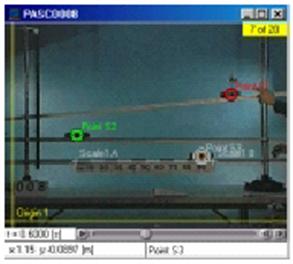
3 Results
The most important findings and observations based on the pre- and post-questionnaire are summarized in Table 1
Table 1
|
|
Subject |
|
1 |
2 |
3 |
4 |
5 |
||
|
1 |
Using only 0-2 random pairs to find the rate of change of the data for a list of 20 numbers, even though it was not requested |
Pre |
|
¥ |
¥ |
¡ |
¡ |
||
|
Post |
|
|
¥ |
|
|
||||
|
2 |
Ability to identify points of intersection of two or more curves on a graph |
Pre |
¡ |
|
¥ |
|
¡ |
||
|
Post |
¡ |
¥ |
¥ |
¥ |
¡ |
||||
|
3 |
Ability to name points of intersection of two or more curves on a graph |
Pre |
¥ |
|
|
|
¥ |
||
|
Post |
¥ |
¥ |
¥ |
¡ |
|
||||
|
4 |
Comparing – crosschecking the truth of information given at the questionnaire with the graphs displayed |
Pre |
¥ |
|
|
|
¥ |
||
|
Post |
¥ |
|
¡ |
¥ |
¥ |
||||
|
5 |
Using the corresponding data table to answer questions about graphs |
Pre |
|
|
|
|
™ |
||
|
Post |
|
¥ |
|
¥ |
¡ |
||||
|
6 |
Prediction of the consequences of a parallel transportation and a rotation of the Frame of Reference regarding position |
Pre |
¥ |
|
¥ |
|
|
||
|
Post |
¥ |
|
¥ |
¡ |
¡ |
||||
|
7 |
Prediction of the consequences of a parallel transportation of the Frame of Reference regarding velocity |
Pre |
|
|
|
|
|
||
|
Post |
¥ |
|
¡ |
¡ |
|
||||
|
8 |
Prediction of the consequences of a rotation of the Frame of Reference regarding velocity |
Pre |
|
|
|
™ |
|
||
|
Post |
¡ |
¡ |
¡ |
™ |
¥ |
||||
|
|
¥ Represents success |
¡ Represents partial success |
|||||||
Analysis of the results
The analysis of the results is based primarily on students’ answers on the pre- and post questionnaire and in part at the notes kept during the sessions with the students.
1) Prior to using VideoPoint, students were asked to read a table which consisted of 20 measurements of the x and y coordinate (taken every 0.1 seconds) of three objects moving simultaneously. In four out of five cases the students tried to estimate the rate of change for x and y, even though that was not requested. Their estimations were either based on mental or written calculations. In the case of written calculations no more than two pairs of numbers were used.
This effort to perform mental or “rough” calculations has been abandoned after they had interacted with VideoPoint in three out of four of the cases. It is our hypothesis that VideoPoint helped them realize that the data presented to them in the table was not of abstract form but represented quantities with physical meaning. Using VideoPoint a link was made, between the data in the table and the real motion event. Thus, they realized that no “generalized” or “rough” comments could be made about those coordinates. In other words, they understood that it is impossible to mentally or “roughly” find the rate of change of such a quantity when one has 20 successive measurements in time.
2) Prior to using VideoPoint, students were asked to identify any points of intersection of three curves displayed in one graph. Only one out of the five was successful in identifying the two intersection points of these three curves. Two more were partially successful as they identified one of the two intersection points. The remaining two were completely unsuccessful. It is very interesting to observe that these two had successfully completed this task after having interacted with VideoPoint!
This result is unexpected and further research is required in order to justify this observation. One possible explanation is that the “mental” interpolation of the three curves is successfully performed after using VideoPoint, because students had a more concrete and uniform image concept regarding the motion of the three objects.
3) Extending observation two, we see that only two out of the three students that were able to identify one or two intersection points of the three graphs, named those points, using either their coordinates on the given graphical representation or by associating them with the corresponding video frame. Being able to name a point on a coordinate system is an important task that students should master after being taught coordinate systems. The remaining three students that were not able to name the intersection points prior to using VideoPoint are successful after having used it. This was an expected difference in performance. A possible justification is that VideoPoint has the dynamic feature of displaying the coordinates (in relation to the given graphical representation) of the user’s mouse index when it is within the boundaries of a graphical representation. When students answered to that question with the aid of VideoPoint they inserted their mouse index in the graphical representation and over the intersecting point and thus they were able to name the two points using their coordinates.
The above change in performance is an indication of how VideoPoint can be used both to enhance students’ understanding of the concept of coordinates on a coordinate system and to help them overcome the common misconception that “the horizontal axis of a coordinate system is always used to represent x and the vertical to represent y”.
4) For the 3 moving objects a graph of the x-coordinate of velocity versus time was given to the students. As two of the objects were moving to the opposite of the positive direction of the x-axis of the Frame of Reference their algebraic value was a negative number. Students were asked to describe the motion of the three objects by interpreting the meaning of the negative values for velocity. We did not receive satisfactory answers to this question; so further research on this finding is needed. Though, an interesting reaction was that some of the students noticed that in fact one of the three objects did not have a negative velocity. In particular, prior to interacting with VideoPoint only two out of the five students noticed that one of the objects did not have negative velocity and marked this on their questionnaire. After interaction with VideoPoint, the ratio has gone up to four out of five. The remaining one student showed no difference prior to and after using VideoPoint.
As the graphs presented to the students prior to using VideoPoint were identical to those provided by VideoPoint in the post-examination, we cannot attribute this change to any of VideoPoint’s features. Rather, we can assume that it was the whole activity design that made a difference. Students participating in this activity have a more active role than the one they have when answering a questionnaire on paper. Because of this, we believe, that they were more motivated and more concentrated in their work. Research has shown (Beichner, 1990) that this is the case when students feel more in control of the situation.
The result is that they behave as if they are working on a project of their own and not taking some sort of examination. We also believe that this more active role-control and its outcomes make students be more cautious and suspicious regarding the information given to them.
5) When students were asked to answer questions based on graphs some of them consulted the table in order to provide an answer. This unexpected behavior indicates that perhaps VideoPoint has not helped students improve their understanding of graphs and they resort to the table in order to answer. Another possible explanation, though, is that VideoPoint operates as a link between the different representations of the table and the graphs. Students realize that the table and the graphs both represent a mathematical expression of the motion they observed, so they decide to consult any of the two representations when providing an answer as they are now convinced that they are two versions of the same thing: In both cases they see a mathematical expression of a motion event.
6, 7, 8) We will explain the change in achievement regarding observations 6, 7 and 8 together, as we believe that it is due to the same reasons. It is obvious from these three observations that VideoPoint has the potential to make a big difference in students’ understanding of the concept of the Frame of Reference. Students were much more successful when answering questions regarding the role of the system of reference after using VideoPoint than before.
Based on the results of the pre- and post-questionnaires, but mostly on the interviews, we could say that the reason for this change is the dynamic nature of the Frame of Reference in VideoPoint. The Frame of Reference as presented mathematically, is an abstract concept that cannot be conceptualized unless it has been visualized in a drawing representing a motion event. Thus, comprehension derived from this visualization is not enough to provide students with the ability to make predictions of how equations of motion, graphs and coordinates would change if the Frame of Reference were to rotate or/and change position. VideoPoint may serve as a means for an advanced conceptualization.
In VideoPoint the Frame of Reference is an object of dynamic nature. Students can manipulate it at will and whenever they want and observe how coordinates, graphs, and equations of motion related to it are updated. It is our hypothesis that being able to “experiment” with the Frame of Reference and observe the change it causes to coordinates, graphs and equations of motion, enhances students’ conceptual knowledge on this subject. Students realize that there is a dynamic link between the Frame of Reference’s position and orientation and the way that graphs and tables of coordinates look. Furthermore, by bringing the Frame of Reference to particular positions of “special” interest, such as positioning one of the axes to be parallel to an inclined level, or bringing the x-axis vertically and the y-axis horizontally, they can deal with misconceptions and gain a better understanding and insight to the role of a Frame of Reference.
The students that took part in this research seemed to particularly enjoy the part of moving and rotating the system of reference and noticing the change it causes to the graphs and tables. Most of them made remarks on this that indicate some sort of “insight” regarding this topic when it was demonstrated to them for the first time.
9) At the beginning of this research there was some concern regarding students’ familiarity with computers. Only one out of five students had advanced computer skills. Two had a few and the remaining two had none. It is very encouraging to see that at the end of the activities all five had almost mastered the skills required to use VideoPoint. They could all run VideoPoint, open a movie, collect data, scale the movie, read tables and create graphs. As two of the students struggled with the use of mouse at the first activity it is amazing that after a maximum of five hours they were able to successfully perform the above tasks on their own. Students were themselves surprised by how well they performed on the computer, which increased their self-esteem. They confessed that they had never thought they could do work on the computer so easily. We consider that this feeling of success was a major factor for the increased motivation that they displayed throughout the activities.
References
Beichner, R. J. (1990) The Effect of Simultaneous Motion Presentation and Graph Generation in a Kinematics Labs. Journal of Research in Science Teaching 27(8), 803-815.
Beichner, R. J. (1996) The Impact of Video Motion Analysis on Kinematics Graph Interpretation Skills. American Journal of Physics 64.
Boyd, A., Rubin, A. (1996) Interactive Video: A Bridge Between Motion and Math. International Journal of Computers for Mathematical Learning, 1, 57-93.
Kaput, James, J. (1994) The Representational Roles of Technology in Connecting Mathematics with Authentic Experience. Biehler, R, Scholz, R. W., Straesser, R., and Winkelman, B. (eds.) Mathematics didactics as a scientific discipline, Kluwer.
Steiner, H.-G. (1990) Needed cooperation between science education and mathematics education. ZDM 22(6).
Wicklein, Robert C. and Schell, John W. (1995) Journal of Technology Education, 6(2).
Zollman, D. A., Brungardt, J. (1995) The Influence of Interactive Videodisc Instruction Using Simultaneous-Time Analysis on Kinematics Graphing Skills on High School Physics Students. Journal of Research in Science Teaching, 32(8), 855-869.
Zollman, D. A., Escalada, L. T., Grabhorn, R., (1996) Applications of Interactive Digital Video in a Physics Classroom. Journal of Educational Multimedia and Hypermedia, 5(1), 73-97.
Zollman, D. A., Fuller Robert G. (1994) Teaching and Learning Physics with Interactive Video. Physics Today.
How to use computer-based learning effectively in mathematics
Neil Pitcher
Paisley, Scotland
1 Introduction
By computer-based learning (CBL) we mean computer packages, which set out to provide on-screen learning environments, through which students learn independently in some sense. This includes electronic materials, both for subject content and for assessment. A number of such systems have been available in Mathematics in recent years (Beevers e.a. 1991, Cook 1994, Harding and Quinney 1996).
For the teacher proposing to use a CBL system, it may not be immediately obvious how best to use it. Like paper-based text books, CBL systems tend to include large amounts of information, so in practice students need to be directed carefully to the selected sections that are relevant to the course being taught. Even when directed to the relevant section however, the student may not necessarily interact with the material in a mature way, but may take a superficial approach, by doing the minimum intellectual work perceived as necessary to complete the directed task. The student moves on without the conceptual understanding or the key transferable skills needed to succeed at future stages.
The concern here is with the way in which students read detailed information, particularly from a computer screen. As the world wide web gains ground this is likely to become an increasingly important issue. As teachers we need to stimulate our students to adopt a mature approach to the materials they read. We contend that, if used imaginatively, a CBL system can promote exactly the kind of mature study skills that students need in today’s competitive and rapidly changing world. In this paper we address issues connected with study skills, linked to CBL systems. We take as an exemplar the “Mathwise” system, which is described in the following sections. We present evidence to suggest how learning activities might be planned in order to achieve this.
2 Description of Mathwise
Mathwise (1998) is a CBL package covering university Mathematics for scientists and engineers at levels 1 and 2 (see Harding and Quinney 1996, Pitcher 1998). Its initial version was produced within the Teaching and Learning Technologies Projects, funded by the UK university funding councils. More recently commercial versions have been produced by the Numerical Algorithms Group (see Mathwise 1998, 2000). Mathwise contains more than thirty different mathematical topics, covering Calculus, Algebra and applications.
Each “module” contains exhaustive information, including theory, test sections and interactive exercises, equivalent to the content of about six lectures. Most Mathwise modules also contain an assessment section. Mathwise assessment goes well beyond multiple choice, being based on an engine which allows the user to input answers in algebraic form. The assessment engine is capable of correctly marking algebraically equivalent answers, as it uses code based on the algebraic evaluation of the string entered, comparing with the evaluation of the equivalent correct answer. We have previously reported on evidence suggesting that the use of such a computer-based assessment facility motivates students to interact well with the learning materials in a CBL system (Pitcher e.a. 1999).
However, we have also been concerned to investigate ways in which students can be encouraged to read mathematical content effectively in its own right, even without using the specific testing facilities just described. Is it possible to design a learning activity, which will motivate the students to read detailed mathematical text, hopefully with enthusiasm?
3 Using Mathwise
The Mathwise system contains a large amount of learning material, which is presented by text and mathematical symbols. The student progresses through the material by reading the text and completing interactive exercises. We have reported on the danger of students skimming lightly through text within Mathwise (Pitcher 1998). The problem is that, using such a shallow approach, the student fails to engage fully with the information and concepts presented.
The question of how readily a reader understands mathematical text is has been addressed in the literature (Newton and Merrell 1994), and is not a trivial problem. We suggest that the identification of an appropriate implementation strategy of the CBL system is of the essence. Using a CBL system should provide the student, not only with information specific to the subject being studied, but should also give the student a positive experience of reading information and assimilating it. The difficult question is, how are we to implement a CBL system among students, so that this is achieved? We suggest that one way of doing this is to set students the task of studying a specific topic in depth using the CBL system, and then reporting back on what they have learned. It would be expected that they study the topic in question rather more deeply than most of the other topics within the course.
We have done this in a one-semester course entitled “Linear Algebra with Differential Equations”, using the topic of complex numbers. Complex numbers provide underlying mathematical tools, which arise in different areas of the course. In Linear Algebra a matrix can have complex eigenvalues, resulting in certain distinctive behaviour of a dynamical system. In Differential Equations a solution can exhibit similar behaviour when the roots of the characteristic equation are complex. Thus complex numbers provide an insight into the inter-connectedness of apparently different aspects of Mathematics.
During the winter semester 2000, we set a coursework exercise to students, in which they began by solving two different problems. First they solved a “Vehicle Suspension System” problem, in which they looked at the differential equation, my”+cy’+ky = 0. They were given the task of calculating the minimum value of c needed to give a vibration-free ride. This involved looking at cases where the characteristic equation could have complex roots. Secondly they solved the discrete “population” equations,
xn+1 = 0.5xn + 0.5yn + 0.5
yn+1 = -0.5xn + 0.5yn + 1.
Here the closed form solution contains eigenvalues and eigenvectors that are complex-valued.
We then gave students the following scenario, advising them to obtain information on complex numbers, either from the Mathwise module, “Complex Numbers”, or from a list supplied of library references.
You are an advisor to HM Government. Your department is conducting an inquiry into Mathematics teaching in universities. There has been a proposal to cut back on some of the more theoretical topics. Yesterday a leading businessman hit the headlines when he was quoted as saying, “Studying weird stuff like complex numbers is a waste of time, because it has no practical application.” This has caused a furore. The tabloid press is demanding that complex numbers should be cut from all university Mathematics courses. Your job is to write a briefing report to the Minister for Education, advising him how to respond in an interview with Jeremy Paxman on tomorrow’s edition of Newsnight. Your briefing should include the following:
Make
sure the Minister knows something about how complex numbers arise, the history
of complex numbers, and the main points of the theory, including real and
imaginary parts and Argand diagrams.
Outline
briefly how complex numbers arise in the car suspension problem.
Outline
briefly how complex numbers arise in the population problem.
Give
the minister some “sound-bites”, which are short, high-impact phrases, to
convince the television viewer that complex numbers are a very important part
of university courses in Mathematics.
The idea behind this exercise is to give students a scenario in which they have to use their initiative to report back on information and ideas learned from Mathwise, which contains information on the history, theory and applications of complex numbers.
4 Response to Mathwise
Initial evaluation of Mathwise, alongside another CBL system, was carried out in the SUMSMAN project (Beevers and Scott 1998). It was established that students do find Mathwise easy to use. 83% of students found it “very” or “quite” useful in their studies. They found the explanations clear and the interactive features helpful. They felt that the best uses of Mathwise were to practice a topic just presented in lectures, to review material they were unsure of, and to revise before an assessment. Interestingly however, only 20% thought Mathwise was useful for a first exposure to a topic.
A general conclusion then from these early evaluation exercises was that a CBL system like Mathwise cannot be a stand-alone solution. It would be a mistake to assume that students could automatically profit from such a system without careful guidance from academic staff. However, when seen as one learning tool among others, Mathwise proves popular and effective among students.
When it came to the particular exercise described in the preceding section, the student response was very positive. The students in general performed well and saw the exercise as worthwhile. Although evidence is still being gathered and analysed, we are able to present some initial observations. At the end of the semester, students completed a questionnaire to analyse their “Attitudes to Study”. This questionnaire has been very carefully designed to categorise students into “deep”, strategic” or “surface” learners (Duff 1997). Briefly, a deep learner takes an active interest, relates different ideas and looks for meaning. A strategic learner is determined to excel and invests effort in organising study towards the desired end of succeeding. A surface learner tends to rely on memorising and has difficulty making sense of content and does not seek connections between different ideas.
The “Attitudes to Study” questionnaire contains 30 statements, to which students indicate agreement or otherwise, using a Likert scale. In each question, 2 points were awarded for strong agreement, 1 for agreement, 0 for a neutral response, -1 for disagreement and –2 for strong disagreement. Ten of the statements typify each of the deep, strategic and surface attitudes. The questionnaire was administered at the beginning and at the end of the semester, and the results are now summarised briefly. From the 40 students in the group the average scores were as in Table 1.
|
Semester |
Average attitude score among the |
||
|
“deep” questions |
“strategic” questions |
“surface” questions |
|
|
Start |
0.77 |
0.75 |
0.19 |
|
End |
0.71 |
0.75 |
0.08 |
Table 1: Comparison of average scores, between start and end of semester
A comparison of the averages between the start and end of the semester suggests that this set of students has a mainly deep/strategic approach to study, which has persisted through the semester. Most of the deep learners were found to be strategic as well. Arguably this is the optimal balance in student attitude. It is desirable that students should have a strategic strand to their study attitude, because it is inevitable that many of them do view their studies as a “means towards an end”. If alongside this we manage to promote a deep strand to their study attitude, then we can claim to have been successful in the learning experience we have provided. A few students were more deep than strategic. These tended to enjoy the computer sessions more than traditional classes. We also note that the greatest fall has been in “surface” attitudes.
Although we cannot claim that these broadly positive attitudes to study result from just one exercise that was set, it does seem that the overall scheme of study is being successful in engendering them. It is intended to administer further questionnaires to determine how useful students have found Mathwise itself, compared with other teaching methods and resources.
5 Conclusion
We have described an imaginative way of using a CBL system to promote positive study attitudes and skills among students. As educators we need to learn what are the most appropriate learning and teaching methods connected with such technology, whose availability is increasing as the world wide web gains ground. The Mathwise system is currently available only on CD-ROM, but it is important that the educational lessons are learnt and carried forward into the new technologies that are emerging. As more research is carried out, based on existing computer tools, future developments have the opportunity to proceed in informed ways.
Mathwise is proving to be an effective learning environment, if used carefully and imaginatively. It can be used in a range of different ways, including information gathering, consolidation of lecture material, revision and assessment. Further research is needed to quantify the effectiveness of the various approaches. Mathwise is used in many UK universities. There is a community of users, called the “Mathwise User Group”
http://mat-nt2.bham.ac.uk/mwug/
which publishes a newsletter and holds regular workshops and other events.
References
Beevers C. E., Cherry B. S., Foster M. G., McGuire G. R. (1991) Software Tools for Computer-Aided Learning in Mathematics. Ashgate.
Beevers C E and Scott T D (1998) SUMSMAN – Collaboration between Scottish Universities. Proc. Tenth Intern. Conf. on Technology and Collegiate Mathematics. Chicago, 41-44.
Cook J. (1994) Bridge the Gap with CALMAT. Proc. Seventh Annual International Conference on Technology in Collegiate Mathematics, 93-96.
Duff, A. (1997) A Note on the Reliability and validity of a 30-Item version of Entwistle and Tait’s revised Approaches to Studying Inventory. British Journal of Educational Psychology 67, 529-539.
Harding R., Quinney D. (1996) Mathwise and the UK Mathematics Courseware Consortium. Active Learning 4, 53.
Mathwise Pre-Calculus and Calculus CD (1998, 2000), Numerical Algorithms Group. Oxford.
Newton D. P., Merrell C. H. (1994) Words that count: communicating with mathematical text. Int. J Math. Educ. Sci., Technol. 25, 3, 457-462.
Pitcher N. (1998) Educational Software in Mathematics: Developing and Using a Mathwise Module. Int. J Math. Educ. Sci., Technol. 29, 5, 709-720.
Pitcher N., Beevers C. E., Goldfinch J. (1999) Computer-Based Assessment: Beyond Multiple Choice. Proc. Fourth International Conference on Technology in Mathematics Teaching. Plymouth.
The visualisation of parameters
Carel van de Giessen
Silvolde, The Netherlands
2. The introduction of parameters
4. Visualising parameters by means of software
5. Examples of the use of the sliding parameter option
The
concept of parameter is difficult to grasp for students in secondary schools.
One
of the reasons that problems arise is the mathematical level needed to
understand a parameter. Understanding a family of parameters requires not only
understanding the concept of parameter but also a clear image of the structure
of a set of graphs. For concept development this is a complex introduction.
In
this paper a different introduction of the parameter will be discussed: The
parameter in a dynamic role investigating graphs. Some recent classroom
experiences will illustrate this approach.
1 The meanings of a letter
The meaning of a letter in a mathematical expression in general depends on the kind of mathematical expression: an equation or a formula. Usiskin (1988) classified the different roles a letter can have as unknown, general number, variable, parameter. Furinghetti and Paola (1994) concluded that the majority of the students they surveyed, had difficulty in expressing the difference between unknown, variable and parameter. Bills (2001) showed how the meanings attached to literal symbols can shift during problem solving procedures.
Here are a few examples to illustrate this.
In
the formula y = 3x2+7x the letter x is considered to be the
independent variable and the letter y the dependent, a matter of convention.
In
the equation 8 = 3x2+7x the letter x has changed into
‘unknown’ which has to be solved
In
the formula y = ax2+7x a third letter appears generally referred to
as parameter, although this actually depends on the structure of the formula
and of the context from which it is derived.
In Realistic Mathematics Education, important in Dutch mathematics education, the learning of mathematics starts from situations that students perceive as realistic. Within a realistic context it is very natural to use word variables instead of letters. The Babylonians already did this. If variables are word variables then formulas become word formulas. In word formulas the relationship between independent and dependent variable is better understood by young students than in abstract formulas. S/he easily gets the feeling of “which one is changing first and which one is following the changes”. The context makes a contribution to that too. In the formula
distance = 3*time2 + 7*time
the variables are less abstract than in
y = 3x2+7x
Gradually the formula can become
distance = 3*t2 + 7*t or d = 3*t2 + 7*t.
2 The introduction of parameters
A handy definition of parameter at first acquaintance is not so easy.
A first introduction of parameter describing a parameter as “a constant that may change” will usually be accepted by the students though the phrase itself is a ‘contradictio in terminis’.
There rests the problem of which letter is the variable and which ones are the variables. The mere use of literal symbols, x and y for the variables and a,b,c,.. for the parameters is not sufficient. To be able to handle a parameter the students must see the structure of the formula, for instance see that y = 2x+10 and y = 8–3x belong to the same type of function.
Firstly the structure of the formula has to be recognised, before the role of the third letter as a parameter can be seen. Parameter has a higher mathematical level than variable. In order to understand parameter the student should have incorporated the concept of variable.
Recognizing the structure of a formula and the role of a parameter in a formula, word formulas and word parameters can be of some help.
An example of an introduction using word variables and word parameter:
Let’s assume that the price of a taxiride is found from the formula
price = 2*time+10.
In this formula the price is in euros and the time in minutes. The number 2 indicates the tariff in euro per minute and the number 10 the basic price of a ride.
In taxis there is a taximeter, though different tariffs in different towns. The taximeter, that is the type of formula, which is a linear one, is the same in all taxis. Only the tariff and the basic price have to be changed. Hence the parameter formula becomes
price = tariff*time+basic price.
A formula like
p = tariff*t + basis or y = slope*x + intercept
clarifies the distinct roles of variables and parameters. In contexts the parameter often functions as a kind of regulator.
3 Roles of parameters
In literature three types of parameters are described by Drijvers (2001): placeholder, changing quantity, generalizer. Hitherto the placeholder and generalizer have been paid more attention to than the changing quantity, probably because it was relatively easy to visualise them. Here the three roles of a parameter will be discussed.
Placeholder
In the role of placeholder the parameter gets specific values one by one. To each of the values belongs a graph, also one at a time. The character of the parameter in this role is a static one, the change of value progresses by leaps and bounds and rather than at random.
In solving problems containing a parameter the role of placeholder seems less suitable because after a short, in a trial-and-error-process the student may have forgotten what s/he is doing and thus will lose hold of the problem.
The static role also shows in generic formulas like y = ax2+bx+c or y = b*gt, where, by means of an index, values can be assigned. The importance of a placeholder lies in the introduction of the idea of parameter but mainly in generic notation of formulas.
Generalizer
In the role of generalizer the parameter is assigned a set of values. To this set, often integers, belongs a sheaf of graphs, also called a family of graphs. The family portrait will contain all the members of the family. The word family suggests that the graphs will have the same looks, though that is not the case of course.
The concept of parameter is suited for thinking about structures and sheaves, but, the other way round, sheaves are less suited for learning about parameters.
The concept of sheaves comes after parameter, a higher level of understanding is needed, and therefore the role of generalizer is not so good to acquaint oneself with parameter. The generalizer and the sheaves coming with it are valuable applications.
Some didactical dangers are hidden in the role of generalizer:
the
student sees the parameter as a sheaf of graphs, which is not hard to imagine;
there is the risk of the concept of parameter and the concept of sheaf being
identified
the
student confuses the serial number of a specific graph of the sheaf with the
value of the parameter.
the
student may wonder why this set, why integers, why this sequence, is there a
mathematical but hidden goal?
as
for problem solving with the help of sheaves the student does not see that the
point is a specific value and not a sheaf.
Changing quantity, the sliding parameter
In the role of changing quantity the parameter dynamically walks through a set of values. There is a graph for each value. As the parameter changes gradually so will the graph. That is to say when you are dealing with nice functions, but dramatic things may happen while the parameter is changing gradually.
For this parameter role we have come up with the term “sliding parameter” (Blokland van, Giessen van de, Tall, 2001) because this term shows what the parameter is doing and also the effect on the graph (most of the times). It is therefore impossible to make the dynamics of this parameter visible on a piece of paper or blackboard. On modern computers the dynamic change of value and of the resulting graph is not so difficult to realise. On the screen the parameter value can be changed by hand or automatically; the graph will change accordingly and one can see what is happening.
The sliding parameter appeals to the students because of the dynamics that is in it. Change is an aspect of life and this goes for math as well.
In three pictures the different roles of the parameter ‘a’ in the formula y = x(a–x)+b can be visualised: the placeholder as one single spout, the generalizer as a fountain, the sliding parameter as a playable spout. Fig. 1 illustrates this.
|
|
|
|
|
Fig. 1: Roles of a parameter |
||
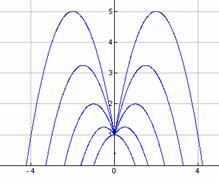
4 Visualising parameters by means of software
If one uses word variables and word parameters in schoolbooks one should use a plotter that can do the same. The programs PlotFormula and Graphic Calculus are graph plotters based on the ideas of David Tall and designed for mathematics education. In both programs there is the sliding parameter and the family parameter. Here some aspects of PlotFormula will be mentioned briefly because this program supports word variables and word parameters.
In the Graphing-option a formula can be entered. The variables may be words or letters, the only, yet small restrictions are some reserved words for instance SIN and INT (see Fig. 2 and 3). The variables are put along the axes. Using word variables units are logical, though optional. All three roles of the parameter as discussed before can be shown.
The placeholder works by simply entering some formulas, each with a specific value of the parameter(s). The graphs are drawn or removed by browsing in the formulas listed on the screen.
|
|
|
|
Fig. 2: Entering a new formula |
Fig. 3: Parameter selection |
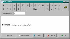
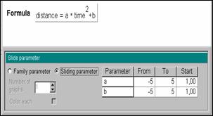
When entering a formula there is a option “Parameter”. By choosing this option a window will appear to choose either the family parameter or the sliding parameter.
The family parameter needs a value to start with, a step and a number for the amount of graphs to be plotted. Moreover each graph can have its own colour. After making these selections and clicking “ok” the sheaf will be shown.
The sliding parameter needs a domain of parameter values. This can be arranged too, but in general the default will do. After clicking ‘ok’ the graph will be shown. At the bottom there is a bar containing the parameter selection mode and the domain of the parameter. The parameter can be changed by hand or automatically. Fig. 4 tells you all about it (On the cdrom SRCPLOTENGDATE.ZIP there’s a demo of PlotFormula and the files going with the examples in this paper).
|
|
|
|
|
|
Fig. 4: Bar for handling the sliding parameter |
|
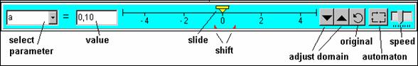
5 Examples of the use of the sliding parameter option
From experiences in the classroom with students of 16-17 years old it becomes clear that the sliding parameter is an option that invites them to play with it. In playing with this parameter the students will find things that motivate them to discuss the results and to do further activities.
The sliding parameter turns out to be a tool in discovering particularities of a graph and so arousing questions about the why of a specific particularity. By investigating a parameter formula the students will find things out themselves or they will be guided through questions.
Because they have made special things on the screen themselves, attention and interest will be drawn. They ask or are asked why they see what they see. Putting the question may lead to understanding and to new questions that may lead to insight, at least that is what we hope.
Seeing, questioning, understanding. The sliding parameter turns out to be a mathematical tool.
Here are some examples form the classroom to illustrate the statements made above.
Investigation on transformation
Starting from standard functions as f(x) = x2, f(x) = 2x, f(x) = sinx etc. the students investigated the behaviour of y = f(x)+a, y = a • f(x), y = f(x+a) and y = f(a • x). Using the sliding parameter they investigated what would happen to the graph and found the vertical and horizontal translations and deformations (see Fig. 5). In some cases it was not possible to distinguish between vertical and horizontal deformation, so a reflection on the formula was needed to explain this.
|
|
|
|
Fig. 5: Transformations of a sinusoid |
|
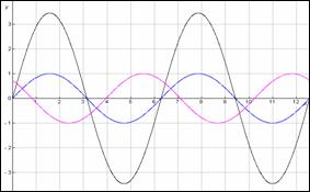
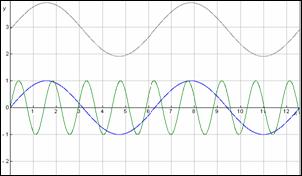
Later on the students did not have problems to explain some rules for differentiating:
y = f(x)+a → dy/dx = f’(x) and y = a • f(x) → dy/dx = a • f’(x)
They referred to the transformations studied before with the help of the sliding parameter.
Investigation on a reciprocal function
The up and down movement of the parabola y = x2+a as a result of changing the parameter a was not a problem for any student. But when looking at the graph of the reciprocal y = 1/(x2+a) they discovered dramatic things. The question was to discuss where and why these things happened and why they happened in the way they did (see Fig. 6).
|
|
|
|
Fig. 6: Graph of function and of reciprocal |
|
Investigation on square root functions
Given were two functions f(x) = (a + x2) and g(x) = (a – x2)
By playing the sliding parameter it showed that one graph is always present whereas the other one disappeared sometimes (see Fig. 7). The question was: why and when is this so? Attention was rapidly drawn but the students should have a good insight in the difference between the variable x and the parameter a. This question proved to be much harder than the previous one.
|
|
|
|
Fig. 7: Graphs of square root functions |
|
Solving problems using a sliding parameter
This example was used for a demonstration of the sliding parameter.
A cheetah is going for lunch when a zebra is crossing.
Will the cheetah, going after the zebra, get hold of the zebra?
First the cheetah has to make a start and then run very fast.
The top speed is high but does not last very long, the cheetah will get tired.
Hence the time-distance-graph consists of three parts: start from 0 to15 seconds, top speed from 15 to 30 seconds and tiredness from 30 to 40 seconds.
This smug zebra runs at a constant speed.
The formulas are in the picture (see Fig. 8). It depends on the beginning distance of zebra and cheetah whether the zebra will fall prey. In finding the safe distance the sliding parameter is a big help.
|
|
|
|
|
|
Fig. 8: Cheetah chasing zebra |
|
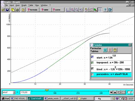
Curve fitting
This example was thought of some students themselves.
Data of a measurement were entered and the graph became a polygon (see Fig. 9).
The students wanted to know whether there was a formula so that the graph fitted this polygon. With the knowledge of standard functions and transformations the students designed a formula containing parameters. Using the sliding parameter the values could be estimated.
|
|
|
|
|
|
Fig. 9: Fitting a curve |
|
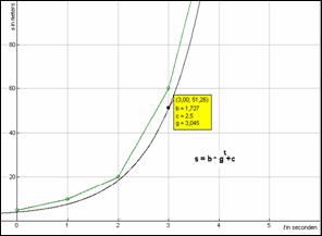
Home made tangents
This example was used in classroom for two reasons.
Firstly to make a parametric equation of a tangent and to demonstrate the result with the sliding parameter. Secondly to demonstrate the family parameter as a survey of what the sliding parameter had done.
Starting with a point (3, 9) on the parabola y = x2, the students found the slope to be 6 and the tangent y = 6x–9 . Then the point (3, 9) was “parametrised” into the point (p, p2) and was derived that the arbitrary tangent on the graph of y = x2 will have the equation y = 2px– p2 where p is the parameter denoting the x-co-ordinate of a dot on the graph.
Using the sliding parameter this will give a walking tangent on the parabola (see Fig. 10).
Using the family parameter this will give a sheaf of tangents enveloping the parabola.
|
|
|
|
Fig. 10: Tangents on a parabola |
|
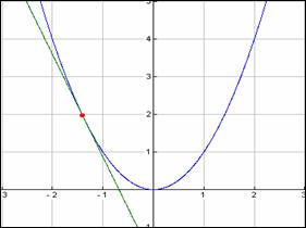
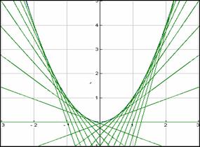
6 Conclusion
The concept of parameter is difficult to grasp for students in secondary schools.
One reason is the difference between variable and parameter. Word parameters in formulas can help students to distinguish between variable and parameter.
Another reason is the mathematical level needed to understand a parameter. Three roles of parameters are described: placeholder, changing quantity and generalizer. The placeholder and generalizer play a static role. The generalizer, visualised by a sheaf of graphs, is possibly better suited for structures and is less suited for introducing parameter.
The sliding parameter restoring changing quantities, is a dynamic option appealing to students. One graph at a time, but the parameter and so the graph can be changed interactively. The sliding parameter offers a lot of didactical advantages introducing parameter as well as working with parameters at a higher level. The sliding parameter can play a role in investigating graphs and solving problems.
References
Blokland P., v. Giessen, C. v. de, Tall. D. (2001) PlotFormula, Graphic Calculus VUSoft. Amsterdam
Bills, L. (2001) Shifts in the meanings of literal symbols. Heuvel-Panhuizen, M. v.d. (ed.) Proc. 25th Conf. on the Psychology of Mathematics Education. Utrecht, The Netherlands, 161.
Drijvers, P. (2001) The concept of parameter in a computer algebra environment. Accepted for publication in: Proc. of the 25th Conference ofr the PME.
Furinghetti, F. and Paola, D. (1994) Parameters, unknowns and variables; a little difference? Proc. of the 18th PME. University of Lisbon.
Usiskin, Z (1988) Conceptions of school algebra and uses of variables. Coxford, A.F. (ed..) The ideas of algebra, K-12. 1988 Yearbook of the NCTM. NCTM, Reston, VA, 8-19.
Note
A demo version of Plotformula is on the CD: SRCPLOTENGDATE.ZIP
Functional algebra
with the use of the graphing calculator
Henk van der Kooij
Utrecht, The Netherlands
1. Difficulties in the learning of algebra
2. Formal algebra and the graphing calculator
3. The final exam: Solving problems with use of the GC
4. A planing machine and the GC
Through a curriculum reform project for vocational education at senior high school level (age 16 - 20), a new mathematics program is designed with two main aims: making mathematics really supportive for the engineering courses and integrating ICT tools in the learning process as well as in assessment.
The students who attend these courses finished junior high school on the lowest level of the three possible streams in junior high in Holland, which means that on the average they are poor achievers in algebra. Instead of putting them back again on the same track that they already failed, it was decided to look for alternative approaches to algebra and for alternative ways of solving problems that, as paper and pencil work, asks for algebraic manipulative skills. For both aspects, the graphing calculator was used as the main IT tool. In this paper, the didactics and technical choices will be presented, followed by work of students on a national exam where the use of the GC was allowed for solving problems. Finally some of the recent papers on the use of the GC will be discussed in the light of our findings.
1 Difficulties in the learning of algebra
The TWIN project (Techniek = engineering, Wiskunde = mathematics, ICT, Natuurkunde = science) is a reform project, meant to design new programs for mathematics and science for vocational courses (engineering) in The Netherlands. Students enter these courses after finishing junior high school at the age of 16. In junior high school there are three main streams: one that will lead to pre-university senior high school, one that leads to the preparation in senior high school for Further Vocational Education (polytechnics) and one that prepares for senior high vocational education. One of the differences between the three levels is the achievement in algebra. Most students that enter the senior vocational courses are coming from the lowest level stream and are not good in using formal algebra. The new programs in junior high are not focused that much on the formal manipulation of algebraic routines. The emphasis is merely on the interchangeability of formulas, tables and graphs, on patterns of growth (linear, exponential, periodic) and on the ways that formulas are built. In the vocational textbooks of engineering however, a lot of traditional algebra is still presented to solve problems. For that reason, mathematics education was emphasizing formal, algorithmic manipulation of algebraic routines in the past. In the TWIN project, an inventory was made first on what mathematical concepts and routines are useful, to make mathematics be supportive for engineering courses and engineering occupational practice.
As far as algebra is involved, the most important findings were:
functions
are relationships between entities with dimensions and units of measurement,
direct
and inverse proportionality are the only and very important power functions in
engineering; general polynomials are hardly found in this field of
applications,
in
relationships, most of the time, there are more than two variables involved.
Based on this inventory and the fact that most students are not very good in algebraic manipulations, two important decisions were made for the design of the new program. The first one was that only the mathematics would be offered that truly supports the engineering subjects and not just for its own (mathematical) sake. The second decision was about the integration of IT tools in both the learning process and in assessment. The most important IT tool is the graphing calculator (GC), in particular the TI 83. Both decisions have far-going consequences for the didactics and the contents of algebra (Van der Kooij, 1999, 2000). In this paper, only the use of the TI 83 will be discussed.
It was found during the project that algebra can make sense to poor achievers when the emphasis is on understanding the concepts instead of algorithmic training on algebraic manipulations. The GC offers many ways to replace (but also to support) algebraic manipulations. In the next paragraph, learning the concept of derivative is presented as an example of how we think that the GC can support the learning of a formal mathematical concept.
2 Formal algebra and the graphing calculator
In this paragraph, it will be discussed how the GC can help in the development of a mathematical concept in a way that is quite different from the traditional pencil and paper approach. The example is about derivatives. The concept of the derivative starts from the linear continuation of a graph, based on the common sense concepts of time-distance and time-speed relationships, first in a graphical way. The following part, taken from the student materials, shows the main idea.
|
4. Yaëll mounts her bike and leaves for a ride. After 4 seconds she has the speed that she wants to keep. The x-t graph shows the first 4 seconds of her ride. a. Draw the graph of her ride, from t = 4 on. b. What is her final (constant) speed? If she did stop accelerating at t = 2, she should have continued with the speed she had at that moment c. Using this information, how can you find her speed at t = 2 with the graph? |
Fig. 1a |
|
The straight lines of 4a and 4c are called the linear continuation (LC) of the graph in a point. The slope of this linear continuation can be interpreted (in this context) as the speed that you had at the moment from which you started to draw the LC. |
|
|
5. At t = 4 a car, moving at a constant speed until that moment, starts to brake until the car is stopped at t = 10. The x-t graph of the braking is shown in this figure. a. At what time did the car pass the sign ‘0 m’? b. What was the speed of the car when it started to brake? c. What is the most apparent difference between this LC and the one of question 4a? |
Fig. 1b |
The phenomenon of the LC is investigated with calculations based on the geometrical visualization through graphs. A simple program for the TI 83 (LINCONT) is also used to find the left- or right side LC in any chosen point of the graph for which the formula is given. Finally, these investigations lead to the well-known expression for the average rate of change (with H>0 for the right side LC and H<0 for the left side LC). This procedure can be used with the GC for any function that is entered in Y1 and for any chosen value of H:
|
|
|
|
|
|
Fig. 2: Numerical derivative with the GC |
|
In this way, too sophisticated algebraic manipulation (including formal treatment of limits) can be avoided and students and teachers can stay closer to the conceptual meaning of the derivative. For a small value of H, the machine already draws a good approximation of the derivative, as is shown in Fig. 2 for the function y = x 3 - 2x.
Further investigations on the derivative, using the available features of the GC, show that the machine cannot always be trusted and that a more strict definition of a derivative is needed. The derivative can be calculated numerically by the GC in two different ways: nDeriv and dy/dx. For special functions, both GC procedures are acting different from the calculations done with the program LINCONT. The GC procedures use a small symmetrical interval around the wanted x. Because dy/dx also makes use of the graph (the cursor is blinking at the right position), this procedure actually checks whether the function is defined for that value of x.
The three ways of finding the derivative for the function y = 1/x in x = 0 result in
no answer at all (dy/dx),
the answer 1000000 (nDeriv)
ERROR: DIVIDE BY 0 (LINCONT)
For the function y = abs(2x) + abs(x-2), the answer given by LINCONT for x = 0 depends on asking for the left side LC (answer -3) or the right side (answer 1). Both procedures of the GC result in the same answer: the average of left and right side derivative (answer -1). Because of these surprises, the need for a more accurate definition of the derivative is apparent. The derivative of a function for x = a exists if (and only if) (1) the function is defined in x = a and (2) left and right side slope both exist and are the same.
Differentiation techniques are presented too, but the students can choose between the use of the GC numerical features or algebra, depending on the accuracy that is needed when solving a problem.
3 The final exam: Solving problems with use of the GC
One of the aims of the TWIN project was to fully integrate the use of IT tools in both the learning process as well as in assessment. It is interesting to look at the first final exam that was presented to the students of the pilot schools to see how the GC was used by students to solve problems. Some questions could not be solved without the use of the GC. Two problems are presented here, together with student work.
|
PROBLEM 3 FLY AWAY Two different types of resistance do influence a flying airplane. The air resistance Fa This resistance is directly proportional to the square of the plane’s speed. For a Boeing 747 the formula is: Fa = 3·v2 with Fa in N and v in m/s. The inductive resistance Fi This resistance decreases with increasing speed. At a higher speed of the plane, the air flow over the wings will be bigger. This air flow is needed to stay up in the air and to enable a plane to fly. Fi is directly proportional to the square of the mass and inversely proportional to the square of the speed. For a Boeing 747 the following formula describes the relationship: with Fi and M in N, and v in m/s The total resistance Ft that a plane experiences, is the sum of the air resistance and the inductive resistance. The most efficient speed is the one at minimal total resistance. The weight at the take off (including the fuel) of a Boeing 747 is 4·106 Newton (mass: 400 tons). Use this weight when answering questions 1, 2 and 3. 9. Use the GC to plot the graphs of Fa , Fi en Ft as functions of v. Use window settings for X: [0,500] and for Y: [0,1000000]. Sketch the graphs on paper. 10. What is the most efficient speed for a Boeing 747? Show your work. 11. Find the derivative of function Ft. Use the derivative to check the answer you found for question 10. During the flight, the mass of the Boeing 747 decreases because of the enormous fuel consumption of about 10 tons per hour. A Boeing 747 flies non-stop from Amsterdam to San Francisco, a flight of about 11 hours. During the whole flight, the pilot wants to keep on flying in the most efficient way. 12. How does he have to change his speed during the flight? Explain how you investigated this problem. |
Question 9 was meant to make the students use the GC to explore the three functions. For question 10 there are at least three ways in which the GC can be used to find an answer:
Use the intersection of the graphs of Y1 and Y2
|
|
Use the minimum of Y3:
|
|
Use the TRACE feature:
|
|
Question 12 is a complex one. It was expected that students who could solve the problem should use one other value of M to find the difference.
|
|
But also, unexpected, solutions were found that went beyond this level:
|
|
Looking at this problem as a whole, it can be concluded that students are able to use the GC to solve problems that do not give away how the answers should be found (questions 10 and 12) and they are capable of finding strategies that involve the use of the GC in a mathematical correct way.
4 A planing machine and the GC
Another problem in the exam was about a driving mechanism that makes a planing machine move to the left (the planing move) and to the right (the back move). The construction (Fig. 3, left) and the schematic picture of that same mechanism ( Fig. 3, right) are given. The crank disc moves counterclockwise.
|
|
|
|
|
|
Fig. 3: Driving mechanism of a planing machine |
|
Part of the problem is presented here.
|
The movement of the planing tool holder can be described with a d - t formula. Fig. 3 (right) shows a schematic picture of the driving mechanism. This picture can be helpful to find the formula. The formula for d is:
15. Explain how this formula can be found, using Fig. 3. Fixed
values are chosen for the length of the crank pin and for the rotational
speed of the disk :
On worksheet 3, you find several copies of this graph. You may use these copies when answering the following questions. 16. Find the measure of angle a (accurate to degrees) at the beginning of the planing move. This driving mechanism has a very nice quality: the speed is almost constant during the planing move. 17. How can this be concluded? 18. Find the speed of the holder, halfway the planing move. 19. For which angle (between 0 and 2p), the holder has its maximum speed? 20. Find the maximum speed. |
One question will be discussed here, because this question asks knowledge of the derivative. The formula is too difficult for the use of the quotient rule. Question 18 is complex: students have to realize that, before finding the speed, they need the correct location at the graph. That is where the graph intersects the horizontal axis downwards. All students did have the program LINCONT in their machine and some of them used it. Four different strategies to find the speed with the GC are given here.
|
|
|
|
|
|
|
|
Four different strategies, all leading to the correct answer. In fact there were at least three more strategies, like using the TRACE feature, partly reasoning and then a calculation with the given formula. This student work shows that the main goal of the new program (students should be able to solve vocational problems with appropriate mathematical tools) is reached. Maybe the most important success factor is the acceptance of the GC as a mathematical tool. Students did show that they are flexible in using the available tools to solve problems in a mathematical appropriate way without drowning in algorithmic formula manipulation.
5 Discussion
Over the last decade, the influences of the graphing calculator on learning algebra of functions are discussed in many papers. Roughly, these articles can be split up in two different groups: the ones that emphasize the danger because a graphing tool should easily cause misconceptions about functions, and the ones that show improvement of students’ conceptual knowledge of functions due to the use of graphical tools.
Studies of the first group, discussed in an overview (Dunham, 2000), are mostly focusing on the problems that are caused by the window format and the discrete nature of (the graphs on) the screen. The supposed misconceptions are mainly: mistakes about slopes because of different scaling on the axes; wrong ideas about (dis)continuity and asymptotes because a graph on the screen is drawn with discrete pixels, and the incompleteness of graphs because of the chosen window setting. I added ‘supposed’ to it, because misconception seems not the right word to use. In my opinion the main problem here is that educators and researchers expect that the use of graphing tools for studying functions should result in the same knowledge and skills as through traditional paper and pencil mathematics education (PPM). Mathematical misconceptions related to the use of graphical tools can only be anticipated if the tool is accepted as a supportive tool for the learning of mathematics, bringing its own qualities. Instead of expecting the same learning outcomes that are reached in PPM, the use of graphing tools should lead to reconsideration of curricular and pedagogical issues.
The second group of papers discusses the improved conceptual knowledge of functions when graphical tools are used in education. These reports discuss well-defined experiments in which graphical tools do support the learning of both the operational concept (a function as a process) as well as the structural concept (a function as an object). The types of problems that are offered in these experiments make full use of the qualities that a graphical tool has to offer: visualizations of algebraically defined relationships. Students who learn the algebra of functions in a graphical tool environment (GTE) are more able to approach problems from a multi-representational perspective (Hollar and Norwood, 1999) than traditionally educated students. One reason for this flexibility of students is the fact that a graphical tool like the TI 83 makes it easy to switch between the three representations of a function: the table, the formula and the graph. Another important reason can be found in the kind of activities that students are dealing with in GTE. In PPM the emphasis is on training algorithmic algebraic routines, where in GTE the “why” is at least as important as the “how” (O’Callaghan, 1998). An important claim of O’Callaghan is that GTE improves students’ attitudes and reduces their anxiety toward mathematics.
When graphical tools are used in the learning of the algebra of functions, it is important to realize that investigations on the typical qualities of the tool (what can it do and how does it work) should be part of the learning process. It should also be realized that the specific qualities of the tool should define the kind of activities that are presented in classroom. The graphing calculator and dynamically defined, interactive Java applets are considered as supportive tools for the learning of algebra. They have the potential of enhancing the flexibility of students to solve problems in which algebra plays a role.
The use of the graphing calculator does not only replace algebra. A closer look shows that there is a lot of algebra included, but in a non traditional way. In traditional programs there was hardly any attention paid to the structure of formulas. In fact, the language aspect of algebra is becoming more important if the use of graphing tools in mathematics education is allowed. For that reason, much attention is paid in the new program on how a formula is built, including notations and rules for algebraic priorities. The training of basic techniques has been de-emphasized, but geometrical aspects of algebra have greater emphasis now: patterns in graphs, like periodicity and symmetry. The features of the TI 83, shown in Fig. 4 are asking for substitution of expressions in formulas, to be able to understand the connection between the (geometry-based) transformations and the influence on the (algebraic) formula and vice versa.
|
|
|
|
|
|
Fig. 4: Geometry-based algebra |
|
Based on the experiences in the project, I see a future for algebra of functions that makes sense to most students. Such a program should
de-emphasize training of basic algorithmic
skills,
pay more attention to the language aspect of
algebra,
use the nice possibilities of graphical tools to
visualize algebraic concepts (the geometry of algebra),
stimulate own investigations by students on
algebraic subjects, supported by graphical tools,
use non-traditional approaches to mathematical
concepts and methods that graphical tools allow
introduce new topics because of the specific
qualities of the tool, like continuous vs discrete and curve fitting
(regression).
References
Dunham, P.H. (2000) Calculators in Mathematics education: Avoiding New Errors. Paper presented to Working Group for Action 11 at the 9th Int. Congress on Math. Ed., Tokyo, Japan.
Hollar, J.C. and Norwood, K. (1999) The Effects of a Graphing-Approach Intermediate Algebra Curriculum on Students’ Understanding of Function. Journal for Research in Mathematics Education, 30, 220-226.
Kooij, H. van der (2000) Mathematics in an Engineering’s Setting: a Real Challenge. Paper presented to Topic Study Group 8 at the 9th Int. Congress on Math. Ed., Tokyo, Japan.
Kooij, H. van der (2000a) What mathematics is left to be learned (and taught) with the Graphing calculator at hand? Paper presented to Working Group for Action 11 at the 9th Int. Congress on Math. Ed., Tokyo, Japan.
Kooij, H. van der (1999) Modelling and Algebra: how ‘pure’ shall we be? Paper presented at the 8th Int. Conference for the Teaching of Mathematical Modelling and Applications, Lisbon, Portugal.
O’Callaghan, B.R. (1998) Computer-Intensive Algebra and Students’ Conceptual Knowledge of Functions. Journal for Research in Mathematics Education, 29,1-40.
Tall, D. (1985) Using computer graphics programs as generic organisers for the concept image of differentiation. In Leen Streefland (ed). Proc. of the Ninth Int. Conf. for the Psychology of Mathematics Education.Freudenthal Institute, the Netherlands, 105-110.
Teague, D.J. (1996). Utilizing Precalculus Experiences with Graphing Calculators: A Local Linearity Approach to Calculus. Paper presented to Working Group 13 at the Int. Congress on Math. Ed., Sevilla, Spain.
Information about the TWIN project can be found on the Internet site www.fi.uu.nl/twin/en
[1] One taught by the author, and the other two by two different colleagues.
[2] “If one changes the tools of thinking available to a child, his mind will have a radically different structure.” (Vygotsky, 1978, 216)
[3] It is possible to use the graphic calculator to enable students to begin to understand the nature of identities and functions, but it needs to be done in a different way from that used in this study. The calculator model remains a concrete one rather than an abstract one.
[4] When asked about prior experience of algebra in a questionnaire, 63% of those who answered the question said they had done some previously, but most qualified this with remarks such as “but I didn’t really understand it”, or “we didn’t do much really”.
[5] Prepared by the author.
[6] Available from the author.
[7] I observed my two colleagues’ classes and one of my colleagues observed my class and me.
[8] Available from the author.
[9] The ALPHA key on a graphic calculator allows the alphabetical stores to be accessed.
[10] Zahra does not appear to realise that any number would do, but thinks of the letters as standing for some specific missing number. This was typical of those students who thought the letters stood for numbers.
[11] On the first questionnaire, she said “a is 1, b is add 2”.
[12] Using the graphic calculator in the way that is described in this paper helps students to see variables as specific but changeable numbers. Moving these students onto a more mature understanding of a variable would need to be considered at a later stage.
[13] See later examples
[14] It is a common misconception at this stage to confuse the operations of squaring and multiplying by 2 (and also to confuse taking the square root with dividing by 2). This would also need further work later.
[15] The one they found very difficult each time was of the form 6a + 2b; the others were of the form 6a+2a and 10b-2b.
[16] Although on this questionnaire, correct answers sometimes do not mean the interpretation of the letters was correct: Emilie gave three correct answers, but said the letters stood for apples and bananas.
[17] A question from one of the homework sheets.