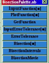
Special Group 5:
Traditional programming - In the age of CAS
Karl Josef Fuchs
Salzburg, Austria
|
Taylor Series and finding zeros with Mathematica and Derive |
|
|
Programming in the age of CAS |
|
|
Problem—Analysis—Encoding—Testing: About program and data structures |
|
|
Programming principles for mathematics and engineering students |
|
|
The digraph-CAS-environment and corresponding elementary programming concepts |
|
|
Combining CAS with authoring systems to create flexible learning environments |
1 Introduction
It was in the middle of summer when we met in the beautiful city of Klagenfurt. The most powerful environment of its university, the beautiful weather in combination with the social activities the organizers had arranged for us and the charisma of the colleagues in our special group were the base for a fruitful discussion throughout the whole week. An overview of the main parts of the discussion is given afterwards. References are included when no paper is added to this overview.
2 Discussion
Programming in the age of CAS
The discussion was opened by my lecture about the importance of traditional programming. In the beginning I pointed out‚ how much programming (knowledge / skills) a mathematics teacher must have in the age of computer algebra. Reasons for the motivation and necessity of this question were given. Different accents in defining the term of programming finally led to the essential argument: Fundamental ideas such as algorithm, function or modelling are very important for the definition of programming in a state of art. And these principles are well-accepted ideas in mathematics.
Programming principles for mathematics/engineering students
Judy Hector pointed out that problem - solving is not a linear process but a five step iterative process. In her college programming courses she starts with elementary algebra problems such as solving a quadratic equation but from the very beginning she has been aware of following the single steps of problem - solving (including discussion about input / output data, hand simulation of partial solutions, coding and testing). Graphical representations are an integral part when developing algorithms. Elementary algebra problems finally lead to more sophisticated problems about logic, calculus or dynamical systems (rabbits / wolves).
The Digraph-CAS-environment and corresponding elementary programming concepts
Wolfgang Lindner focussed on the importance of programming when using a Computer Algebra System in linear algebra. His real life problem about modelling a net of bus connections in Sicily was most impressive and very going along with the characterization of programming as Implementation of abstract models with the aim to visualize and to prove the character of the models through simulation. On one hand Wolfgang Lindner pointed out that programming is equal to Implementing Functions (especially when using CAS) and that clarifying the data-structures is most important in the beginning of a coding - process but on the other hand he added the new aspect that modelling always means reduction and abstraction.
How can we combine the CAS with authoring system tools to create a flexible learning environment
Once again Csaba Savari and Mihaly Klincsik pointed out the iterative character of a step-by-step solving-process in their toolbook-philosophy. Additionally they made a ‚look behind the curtain‘ possible for our discussion group. The ‚look behind the curtain‘ means the following: We could
 see the data structures which were used for the
implementation (polynomial approximations, vectors, lists),
see the data structures which were used for the
implementation (polynomial approximations, vectors, lists),
see the procedures (and the parameters) in the
simplex package,
the control structures of the algorithms they
were using in the presented problems,
the graphical representations of the modules (in
the transportation problem)
Taylor Series and finding zeros with Mathematica and Derive
Alfred Dominik (BORG Salzburg) felt sorry for the weak programming skills of his grammar school students when implementing functions hidden behind the Mathematica - Palettes and the chained Derive - functions although his students have had obligatory computer science lessons for many years. But these computer science lessons more focus on the use of text processing systems, presentation software than on programming (skills / abilities). Once again we could discuss the importance of the idea of the function (with different parameters) and the idea of the data structure when defining programming as a process, which aims at the implementation of algorithms and data structures on computers. Executable tested programs where called ‘movies’ by Alfred Dominik.
Problem – Analysis – Encoding – Testing - About program and data structures
Eva Vasarhélyi (Eotvos Lorand University Budapest) and I presented a short introductory material for procedural programming with a hand-held-technology-computer. The process is organized around a real life problem (the post-office) and the reader follows the iterative steps of analysis, encoding and testing. In the end a summary on the introduced data and control structures is given as a leaflet, which can be handed out to the students. An additional aspect is the ‘genetic structure’ of the presented material, which means that each further step is provoked by a new step of refinement.
Taylor Series and finding zeros with
Mathematica and Derive
Alfred Dominik
Salzburg, Austria
1. Fix point iteration with Derive and Mathematica
2. Finding zeros with the regula falsi
3. Taylor series with Mathematica
This paper intends to show, how Mathematica and Derive can be used for finding zeros of functions, visualization of fix point iteration processes and Taylor series. Many papers are concerned with algorithms for using Derive in calculus (e.g. Fuchs 1998; Aspetsberger, Fuchs, Heugl, Klinger 1994; Berry et al 1993; Scheu 1992). In Austria we have several approaches to use Mathematica in secondary schools (Dominik and Fuchs 1999; 2000; Wilding and Simonovits 1997; Simonovits 2000). I tried to use both Mathematica and Derive for teaching Taylor series and iteration processes in order to compare the facilities of the two CAS, a valuation of the comparison is let to the reader.
1 Fix point iteration with Derive and Mathematica
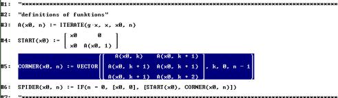
According to an idea from Fuchs (1988) and Schweiger (1993) I used the Spinne (spider) procedure to visualize the fix point iteration method to find zeros.
|
|
|
Fig. 1 |
|
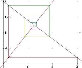
Example: We solved –1.6 x + 2 = 0 to visualize the iteration method. Program call Spider(3,10) produced a sequence of 10 iterations of the equivalent iteration function –0.6 x + 2 starting with n0 = 3. The result is plotted in Fig. 2. The other zero can be found in the same way. |
|
|||
|
|
Fig. 2 |
|||
|
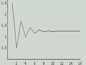
With Mathematica you can do the same things, but in addition you can animate these graphs, so you can see what is going on during the iteration process. We solved example 1 using a Mathematica Palette (for an explanation of palettes see Dominik and Fuchs 1999; 2000). The procedures are listed below. We created two animated plots (Fig. 3 and 4) |
|
|||
|
|
Fig. 3: IterationPlot[0,3] |
|||
|
IterationMovie yields a movie (Fig. 4). |
|
|||
|
|
Fig. 4 |
Procedures
IterationList[a_,b_]:=
Table[Part[NestList[f,a,b],i],{i,1,Length[NestList[f,a,b]]}]
IterationPlot[a_,b_]:=ListPlot[list,PlotRange
->{{0,Length[list]},{a,b}},PlotJoined->True];
StoreList[a_]:=list=a
spiderpoints[k_]:=
Flatten[Table[{{Part[list,i],Part[list,i+1]},{Part[list,i+1],
Part[list,i+1]},{Part[list,i+1],Part[list,i+2]}},{i,1,k}],1]
IterationMovie:=
Do[ListPlot[spiderpoints[k],PlotRange->{{0,Max[list]},{0,Max[list]}},
PlotJoined->True],{k,1,Length[list]-2}]
SpiderFunction:=
ListPlot[spiderpoints[Length[list]-2],
PlotRange->{{0,Max[list]},{0,Max[list]}},PlotJoined->True]
Plotf=Plot[f[x],{x,0,Max[list]}];
Plotx=Plot[x,{x,0,Max[list]}];
ShowWholeWeb:=Show[{SpiderFunction,Plotf,Plotx}]
ShowFunctionAndMedian:=Plot[{f[x],x},{x,0,2*Part[NSolve[f[x]==x],1,1,2]}];
2 Finding zeros with the regula falsi
|
According to Fuchs (1998) we defined a Derive procedure “bisec” to find zeros with the regula falsi: bisec(a, b) := if ( abs (a-b) < 10-4, a , if ( f( (a+b)/2 )*f(a) < 0, bisec(a, (a+b)/2) , bisec((a+b)/2, b))) This strategy worked very well with several functions, so we decided to create a Mathematica palette for further investigation. |
|
|||
|
|
Fig. 5 |
Procedures
Bisection[a_,b_]:=(i++;m[i,1]=N[a];m[i,2]=N[b];
If[Abs[a-b]<ErrorTolerance,
( Print[N[(a+b)/2]];j=i;i=0;),
If[f[(a+b)/2]*f[a]<0,
Bisection[a,(a+b)/2],
Bisection[(a+b)/2,b]]]);
i=0; (global notebook feature for safety reasons)
InputFunction:=f[x]
InputErrorTolerance[a_]:=fe=a;
ErrorTolerance:=fe
NumerischesErgebnis[a_]:=N[a]
BisectionIntervals:=
Table[{"Interval Number:",k,m[k,1],m[k,2],
":Estimated Zero",(m[k,1]+m[k,2])/2},{k,1,j}]//TableForm
FunctionsPlot:=Plot[f[x],{x,-5,5},DisplayFunction->Identity]
listplotlinks[i_]:=
ListPlot[{{m[i,1],-5},{m[i,1],5}},PlotJoined->True,
PlotRange->{{m[1,1]-1,m[1,2]+1},{-15,15}},DisplayFunction->Identity]
listplotrechts[i_]:=
ListPlot[{{m[i,2],-5},{m[i,2],5}},PlotRange->{{m[1,1]-1,m[1,2]+1},{-15,15}},
PlotJoined->True,DisplayFunction->Identity]
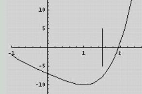
BisectionMovie:=
Do[Show[listplotlinks[i],listplotrechts[i],FunctionsPlot,
DisplayFunction->$DisplayFunction],{i,1,j}]
|
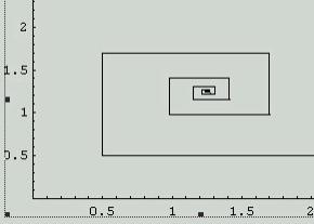
With these palette procedures you can, for instance, create an animated film that shows the convergence of the bisection intervals, Fig. 6. |
|
|||
|
|
Fig. 6 |
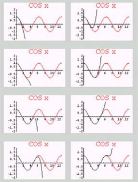
3 Taylor series with Mathematica
|
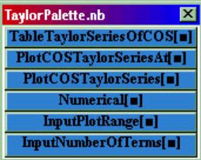
We used this palette to investigate Taylor series, using the Taylor series of COS (x) to understand what’s going on. |
|
|||
|
|
Fig. 7 |
|
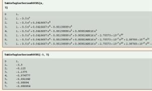
In Fig. 8 we created a table of the first 7 terms the Taylor series of COS (x), then we substituted x=-3 to get a Taylor approximation of COS (-3). With PlotCOSTaylorSeries[7] we created a film to show the “global” convergence of the Taylor series; for this paper I chose to put the sequences of the film into a graphics array (Fig. 9)
|
|
|
Fig. 8 |
Fig. 9 |
Procedures
Taylorcos[x_,n_]:=Sum[x^(2*k)/(2*k)!*(-1)^k,{k,0,n}]
cosplot:=Plot[Cos[x],{x,0,4*Pi},PlotRange->{-2,2}, PlotStyle ->
RGBColor[1, 0, 0],Background->RGBColor[1,1,1],
PlotLabel->
StyleForm[COS(x),FontSize\[Rule]20,FontColor->RGBColor[1,0,0]]];
cosplot2:=Plot[Cos[x],{x,0,4*Pi},PlotRange->{-4,4}, PlotStyle ->
RGBColor[1, 0, 0],Background->RGBColor[1,1,1],DisplayFunction->Identity, PlotLabel->
StyleForm[COS(x),FontSize\[Rule]20,FontColor->RGBColor[1,0,0]]];
g[x_,i_]:=Table[{k,Taylorcos[x,k]},{k,0,i}]
InputPlotRange[a_,b_,c_,d_]:=Zeichenbereich ={{a,b},{c,d}}
TableTaylorSeriesOfCOS[x_,i_]:=TableForm[N[g[x,i]]]
PlotCOSTaylorSeriesAt[x_]:=
Do[ListPlot[g[x,i],PlotJoined->True,PlotRange->Zeichenbereich],{i,0,
Termanzahl}]
InputNumberOfTerms[a_]:=Termanzahl=a
g[x_,i_]:=Table[{k,Taylorcos[x,k]},{k,0,i}]
PlotCOSTaylorSeries[n_]:=
Do[Show[cosplot2,p[i],DisplayFunction\[Rule]$DisplayFunction],{i,1,n}]
p[i_]:=Plot[Taylorcos[x,i],{x,0,4*Pi},DisplayFunction\[Rule]Identity]
q[i_]:=Show[cosplot2,p[i]]
Numerical:=N
4 Conclusion
Mathematica and Derive are valuable tools for iteration processes and Taylor series. They can help students to understand the basic ideas. I did some of the programming (bisec, taylorcos) with the students; some of them felt, this had really nothing to do with mathematics; others liked the transfer of mathematical ideas into CAS procedures. I am convinced, that especially the films helped the students to understand what is going on during an iteration process or to understand the meaning of adding terms of a Taylor series. Also I recognized, that the use of the computer algebra systems had a good influence on the social structure of my school class (15 girls, 12 boys, age 17). Of course, further investigations are needed.
References
Aspetsberger, K., Fuchs, K., Heugl, H. and Klinger, W. (1994) The Austrian Derive Project-Final report. Sonderschrift des BMUK, Wien.
Berry, J.S. e.a. (1993) Learning Mathematics Through DERIVE. Chichester Ellis Horwood Limited
Dominik, A. and Fuchs, K. (1999) Mathematica Palettes – A Methodical Way to Provoke Students Into Using Mathematical Strategies. ICTMT 4. University of Plymouth.
Dominik, A. and Fuchs, K. (2000) Mathematica Palettes – Eine für den mathematisch-naturwissenschaftlichen Unterricht adaptierte/adaptierbare Lernumgebung. ÖMG Schriftenreihe Did. der Math 32.
Fuchs, K.J. (1988) Computeralgebra – Neue Perspektiven im Mathematikunterricht. Habilitationsschrift, Univ. Salzburg.
Scheu, G. (1992) Arbeitsbuch Computeralgebra mit Derive. Dümmler, Bonn.
Schweiger, F. (1993) Chaotische dynamische Systeme. Mathematik im Unterricht 17, 17-45.
Simonovits, R.(2000) Project M@th Desktop. ÖMG Schriftenreihe Did. der Math 32.
Wilding, H.and Simonovits, R. (1997) Visualisierung funktionaler Zusammenhänge mit animierter Graphik in Mathematica – Notebooks. ÖMG Schriftenreihe Did. der Math. 26.
Programming in the age of CAS
Karl Josef Fuchs
Salzburg, Austria
2. Programming – A term’s accents
3. Timeless concepts in programming
The author will concentrate on the basic question of the special group by taking How much programming (knowledge / skills) must a mathematics – teacher have in the age of CAS as their theme. Reasons for the motivation and necessity of this question for the process of teaching mathematics with new technology will be given. Different accents in defining the term of programming will show that fundamental ideas of mathematics such as algorithm, function or modelling are essential parts of these terms.
1 Ongoing and motivation
For many years mathematics – teachers have been carrying informatics
as a subject in Austrian Grammar schools. More and more the teacher-studies in
mathematics at the universities have been adapted to these new requests.
Lectures have been integrated into the curriculum of teacher – studies to make
the teacher-students familiar with programming in at least one program
language. One year ago teacher – studies in informatics were introduced at the
universities in Vienna, Salzburg and Klagenfurt. So once again we will have to
react due to this new situation as teachers in mathematics education
In the eighties and beginning nineties the discussion about the
introduction of computers in a manner appropriate to the children’s‘ age was
dominated by the discussion about the use of the ‚right‘ programming language.
I think everybody remembers the controversy reactions provoked by Seymour
Papert’s book Mindstorms (Papert 1982; Bender 1987). The papers discussing
programming in mathematics – lessons disappeared in such an extent as the
papers in mathematics education focussed on educational models for the use of
Computer Algebra Systems. But for me the question is still vivid: Did the
discussion about programming in mathematics really come to an end or was it
only suppressed?
Starting from the assumption that we can solve most of the problems
in mathematics – lessons with predefined Derive, Maple or Mathematica functions
we will soon be disappointed especially if we decide to go an individual way.
Even implementing new modules (Aspetsberger and Fuchs 1995) by chaining
predefined CAS – functions makes some basic programming skills unavoidable.
Additionally I want to mention that for some years we have the
possibility to bring Computer Algebra Systems into the classroom very easily
with the hand-held technology of the TI-92 or the Cassiopeia Maple Calculator
(see Fuchs and Vasarhélyi 2002, this volume). I think - as being teachers in
mathematics education- we have the obligation to make the teacher-students
familiar with this new technology.
But is programming part of the basic skills we will have to teach them? I want to focus on this question.
2 Programming – A term’s accents
I think that it is profitable to make an overview of different definitions of programming in books of mathematics- or informatics education. Unfortunately all the examples are taken from books written in German. So I decided to translate them into English. I hope that the meanings of the definitions don’t suffer from the translation. Questions like the philosophy of programming, or strategies of programming (the way of Coding – Editing – Debugging), I don’t want to discuss in these statements. The first definition is taken from Jochen Ziegenbalg’s book Algorithmen. He (Ziegenbalg 1996) distinguishes between
“Imperative Programming: A sequence of commands which changes the state of the computer (in general by changing the registers‘ occupying) Functional Programming: Coded functions which transfer arguments to (function) values.”
We can find another definition in the book Informatik für den Lehrer (Informatics for teachers) by Hans W. Haas and Detlef Wildenberg (1982)
“Programming aims at the implementation of algorithms (and data structures) on computers.”
Peter Hubwieser (2000) sees programming in his book Didaktik der Informatik (Informatics Education) as
“Implementation of abstract models with the aim to visualize and to prove the character of the models through simulation.”
A similar definition is given by Gerald Futschek (1990) in his paper informatics as a scientific discipline.
“First the computer scientist draws up a model to solve a given application problem. ... The initial model will be modified stepwise to other models, which will always become more detailed and more formal. This iterative process will be run through until a final model coded in a program language will come out.”
Finally we can find a definition of programming by Gustav Pomberger (1999):
“Programming in the sense of computer science means to formulate a solution to a given task which can be executed by a computer.”
3 Timeless concepts in programming
At the end of the first section, I formulated the question if programming would be an essential part of computer skills teacher-students should be taught. I see the main criteria to answer this question in the different definitions in chapter 1 which means:
Are there any timeless concepts in teaching programming?
Looking back to the definitions we will find the idea of the algorithm. This idea is undoubtedly one of the well-accepted basic concepts in applied mathematics (Reichel 1995). You can find this idea in very different lists of fundamental ideas or concepts of mathematics.
Elmar Cohors-Fresenborg (1987) sees the ideas of the function (or functional dependence), modelling and algorithm standing close together. Functional dependencies between different parameters are recognized in the process of modelling and finally implemented into the computer as algorithms.
Be aware that also Gerald Futschek and Peter Hubwieser see a characteristic of programming in the implementation of models.
In particular this applies to Computer Algebra Systems. See the following examples:
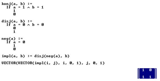
a) Coding and chaining elementary logical functions (coded in DeriveTM)
|
|
|
|
b) Modelling iterative processes numerically (coded in MathematicaTM)
F[x_]:=x+0.3(20-x)
NestList[F,6,20]
{6,10.2,13.14,15.198,16.6386,17.647,18.3529,18.847,
19.1929,19.435,19.6045,19.7232,19.8062,19.8644,19.905,
19.9335,19.9535,19.9674,19.9772,19.984,19.9888}
Hans-Joachim Vollrath (1989) calls functional thinking (in the sense of functional programming) one of the most important ‚didactical stimuli‘ in mathematics education.
|
The idea of the data structures (constants, variables, arrays, sets, lists), which we can find in the definition of Haas and Wildenberg, was seen as fundamental in a paper I presented in 1994 (Fuchs 1994). But also Hans-Christian Reichel (1995) sees a fundamental concept of applied mathematics in the idea of data structures and relations. This discussion of relations will focus on control structures
which are also implemented in Computer Algebra Systems (see the following example coded in MapleTM) tower := proc(a) local result; result := a; for i to 2 do for j from 2 to 9 do print(result); if i=1 then result:= result*j else result := result /j fi od od end |
|
4 Summary
So how can my answer to the question about timeless ideas in programming look like? If you decide to accept the different accents in defining the idea of programming you will also have to accept a lot of timeless ideas, which are fundamental characteristics of these definitions. Whenever you will plan to exclude the discussion of a program language from the curriculum of mathematics teacher-studies there will remain these doubtless fundamental concepts which we still should teach our students even in the age of Computer Algebra Systems.
References
Aspetsberger, K. and Fuchs, K. (1995) Derive im Mathematikunterricht: Zur Organisation von Beobachtungseinheiten; Modultechnik im Mathematikunterricht mit Computeralgebra. Beiträge zum Mathematikunterricht. Franzbecker, Hildesheim, 74-77
Bender, P. (1987) Kritik der LOGO-Philosophie. JMD 8, 3-103
Cohors-Fresenborg, E. (1987) Zur Integration algorithmischer und axiomatischer Denkweisen in den Mathematikunterricht der Klasse 7 des Gymnasiums. Beiträge zum Mathematikunterricht. Franzbecker, Hildesheim, 130-133
Fuchs, K. J. (1994) Didaktik der Informatik: Die Logik fundamentaler Ideen. Medien und Schulpraxis 4+5, 42-45
Fuchs, K. J. (1998) Computeralgebra - Neue Perspektiven im Mathematikunterricht. Thesis Salzburg.
Futschek, G. (1990) Informatik als Wissenschaft. Reiter, Anton Rieder, Albert Didaktik der Informatik. Jugend und Volk, Wien, 2-6
Haas, H. and Wildenberg, D. (1982) Informatik für Lehrer - Band 2: Komplexere Probleme und Didaktik der Schulinformatik. Oldenbourg Verlag, München, Wien
Hubwieser, P. (2000) Didaktik der Informatik. Springer, Berlin, Heidelberg, New York
Lechner, J. (1996) Iteration und Rekursion - Problembeschreibung und Lösungsmethode zugleich. Teaching Mathematics with DERIVE and the TI-92, ZKL-Texte Nr. 2, Münster, 303- 318.
Papert, S. (1982) Mindstorms - Kinder, Computer und Neues Lernen. Birkhäuser.
Pomberger, G. (1999) Prozedurorientierte Programmierung. Rechenberg,
Pomberger, G. (2000) Informatik-Handbuch. Carl Hanser Verlag, München, Wien, 517-528.
Reichel, H.-C. (1995) Fundamentale Ideen der Angewandten Mathematik.Wissenschaftliche Nachrichten, 20-25.
Vollrath, H.-J. (1989) Funktionales Denken. JMD 10, 3-37.
Ziegenbalg, J. (1996) Algorithmen. Texte zur Didaktik der Mathematik. Spektrum, Heidelberg.
Problem – Analysis – Encoding – Testing
About program and data structures
Karl Josef Fuchs and Eva Vasarhélyi
Salzburg, Budapest
First refinement: Organising the input – More about data structures
Second refinement: Modifying the output
The authors will show an example for the use of hand-held CAS-Technology in computer science. From the educational point of view stepwise refining and modification concentrate on the flexible and effective use of basic comments of an imperative programming tool in many different ways.
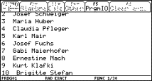
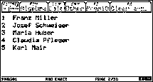
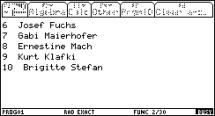
ProblemIn the 10th floor of an office-block are working-rooms numbered from 1 to 10. The following people work in these rooms: 1 Franz Miller 2 Josef Schweiger 3 Maria Huber 4 Claudia Pfleger 5 Karl Mair 6 Josef Fuchs 7 Gabi Maierhofer 8 Ernestine Mach 9 Kurt Klafki 10 Brigitte Stefan Design a program which displays the room number and the name of the office-worker for the ten rooms. |
|
|
|
Fig. 1 |
Analysis
The Analysis of the problem shows that it can be solved by a sequence of commands, which contain numerical and string constants as parameters.
Encoding
We can code the first algorithm (= simple sequence of commands) easily. The TI-92- commands we need are as follows.
problem01a()
Prgm
Disp string(1)&" "&"Franz Miller"
Disp string(2)&" "&"Josef Schweiger"
Disp string(3)&" "&"Maria Huber"
Disp string(4)&" "&"Claudia Pfleger"
Disp string(5)&" "&"Karl Mair"
Disp string(6)&" "&"Josef Fuchs"
Disp string(7)&" "&"Gabi Maierhofer"
Disp string(8)&" "&"Ernestine Mach"
Disp string(9)&" "&"Kurt Klafki"
Disp string(10)&" "&"Brigitte Stefan"
EndPrgm
Comments on the code
In each program line Disp string(10)&" "&"Vorname Nachname“ we connect the room numbers (data structure: numerical constant) and the names of the offices – workers (data structure: string constant). As we only can put constants of the same type together we use the string- function, which changes our numerical constant to a string constant for our code.
TestingStarting the program with problem01a() ¸, the screen looks as Fig. 2a. First refinement: Organising the input – More about data structuresWe see that it is very laborious to enter each room number. The room numbers are of increasing order from 1 to 10 only the names of the office – workers in these rooms are different. |
|
We can shorten the program code (= source code) by the following strategies: We assign all the names to a list (this data structure is also called vector or array) and afterwards we use an iteration command (to count the room numbers from 1 to 10 and fetch the related name of the office – worker from the list.
|
{Franz Müller, |
Josef Schweiger, |
.... , |
Brigitte Stefan} |
|
↑ |
↑ |
|
↑ |
|
Index 1 |
Index 2 |
… |
Index 10 |
Implementing the described strategies leads to the modified code:
problem01b()
Prgm
{"Franz Miller","Josef Schweiger",
"Maria Huber","Claudia Pfleger",
"Karl Mair","Josef Fuchs",
"Gabi Maierhofer","Ernestine Mach",
"Kurt Klafki","Brigitte Stefan"}->name
For i,1,10,1
Disp string(i)&" "&name[i]
EndFor
EndPrgm
Comments on the code
a) The line
{"Franz Miller","Josef Schweiger","Maria Huber",
"Claudia Pfleger","Karl Mair","Josef Fuchs",
"Gabi Maierhofer","Ernestine Mach","Kurt Klafki",
"Brigitte Stefan"}->name
is an assignment. A list of string constants is denoted by name. Each cell of the list can be called by its index (= i).
b) The TI-92-iteration command we use for the implementation is For – EndFor. The iteration variable i (= Index) is a numerical variable. Executing the iteration i is ‚running‘ from 1 to 10 with step 1.
c) When we start the program once again with problem01b()¸, the output on the calculator’s screen will not change.
Second refinement: Modifying the output
We want to make the output on the screen more attractive in the next step. The program should display 5 elements and stop. Entering any key the output screen should be cleaned and the next 5 elements should be displayed.
a) To solve this modified problem we need a command for branching (IF command).
b) Additionally we will need the GetKey()-function, which will prove if any key is pressed. While no key is pressed the GetKey()-function will respond with the value 0.
c) The ‚delay‘ will be implemented by the iteration command While – EndWhile .
d) The command ClrIO is responsible for cleaning the screen.
e) The mod (modulo function) stands for mod (5,a) = {1, 2, 3, 4, 0} with a Î {1, 2, 3, 4, 5}.
These changes lead to the modified code of the second refinement:
problem01c()
Prgm
{"Franz Miller","Josef Schweiger","Maria Huber","Claudia
Pfleger","Karl Mair","Josef Fuchs","Gabi Maierhofer","Ernestine
Mach","Kurt Klafki","Brigitte Stefan"}->name
For i,1,10,1
Disp string(i)&" "&name[i]
If mod(i,5)=0 Then
getKey()->key
While key=0
getKey()->key
EndWhile
ClrIO
EndIf
EndFor
EndPrgm
Starting with problem01c()¸, we get first Fig. 2a. After pressing the ¸-key we get the next 5 names – Fig. 2c.
|
|
|
|
|
|
Fig. 2b |
Fig. 2c |
Third refinement: Open List
In the third modification our program should be able to accept any assigned name of an office – worker to the 10 office rooms.
Therefore we need an open list, which we generate with the newList-function. Each name is entered by the InputStr-command.
The command empl->name[i] shows you how each cell of the list name is filled by the name which the variable. employee (= empl) contains. The iteration is realized by the Loop –EndLoop-iteration command.
The new source code looks like:
problem01d()
Prgm
ClrIO
newList(10)->name
1->i
Loop
InputStr "room"&string(i)&": ",empl
empl->name[i]
i+1->i
If i>10 Then
Exit
EndIf
EndLoop
ClrIO
For i,1,10,1
Disp string(i)&" "&name[i]
If mod(i,5)=0 Then
getKey()->key
While key=0
getKey()->key
EndWhile
ClrIO
EndIf
EndFor
EndPrgm
As we decided to collect the important information of the ongoing process we prepared the following instruction leaflet for the students.
|
A new word requires our concentration. It is the idea of the algorithm which is important to theoretical informatics and which describes the commands and their order, which are necessary to solve a given problem. We have modified our problem in many different ways. Now it is time to summarize the data- and program structures we discussed before 1. Data structuresWhat we learned: a) Objects with a concrete value, which have an evident meaning, are called constants, for example string constant „Karl Mair“, numerical constants 1, 2. b) Objects which consist of a name and a related object are called variables, for example numerical iteration variable i (Name: i, related objects: 1, 2 .. 10); string variable empl (Name: empl, related objects: First name, last name) c) Objects which are built up by the simple objects mentioned in (a) and (b). In our problem lists, arrays or vectors. The built-up-object gets a new name. The simple objects are the components of the new object. |
|
||||||||||||||
|
z. B. name |
|
||||||||||||||
|
Franz Miller |
Josef Schweiger |
Maria Huber |
Claudia Pfleger |
Karl Mair |
Josef Fuchs |
Gabi Maierhofer |
Ernestine Mach |
Kurt Klafki |
Brigitte Stefan |
|
|||||
2. Program structuresWhen summarizing the program structures we heard before we will follow the graphical representation with structograms by Nassi and Shneiderman. In this representation all algorithms can be seen as a combination of the following basic elements. Each element has the shape of a rectangle and is labelled by its characteristic name. a) The process symbol consists of assignments, input and output commands just as of calls of procedures. |
|
||||||||||||||
|
|
Block |
|
TI-92 Code: |
|
|||||||||||
|
|
Disp string(1)&" "&"Franz Miller" |
|
|||||||||||||
b) The decision symbol illustrates branching. |
|
||||||||||||||
|
|
condition |
|
|
||||||||||||
|
|
ß true Ü |
à false Ü |
If condition Then „Then“ body Else „Else“ body |
|
|||||||||||
|
|
body |
body |
|
||||||||||||
|
c) The iteration symbol illustrates an iteration. |
|
||||||||||||||
|
c.1) while symbol (control in the beginning) |
|
||||||||||||||
|
|
While condition true |
While condition body EndWhile |
|
||||||||||||
|
|
|
body |
or For iteration variable, start,end,step body EndFor |
|
|||||||||||
|
|
|
||||||||||||||
|
|
|
||||||||||||||
|
c.2) repeat – until – symbol (control in the end) |
|
||||||||||||||
|
|
|
body |
Loop body (Exit) EndLoop |
||||||||||||
|
until condition true |
|||||||||||||||
|
|
|
|
|||||||||||||
|
|||||||||||||||
Addition: Program design
We can use input/output windows to make programs more attractive. With the Dialog – EndDlog commands we can generate dialog boxes. The Title command specifies the headline of the box. Inputs are implemented by the Request, outputs by the Text command. Our last modification looks like: (The part of the source code which is related to the dialog window is highlighted.)
problem01e()
Prgm
ClrIO
newList(10)->name
1->i
Loop
Dialog
Title "employees in ..."
Request "room"&string(i)&": ",empl
EndDlog
empl->name[i]
i+1->i
If i>10 Then
Exit
EndIf
EndLoop
ClrIO
For i,1,10,1
Dialog
Title "occupied rooms"
Text "room "&string(i)&": "&name[i]
EndDlog
EndFor
EndPrgm
References
Borovcnik, M. (1992) Glücksspiele in Theorie und Praxis. Skriptum zur Lehrerfortbildung, Salzburg.
Caba, H.; Fuchs, K.J. (1989). Informatik Heute 5. Jugend-Verlag, Salzburg.
Caba, H.; Fuchs, K.J. (1992): Versuch einer Methodik und Didaktik des Computereinsatzes im Unterricht. Informatik in der Schule - Informatik für die Schule. Böhlau, Wien.
Fuchs, K.J. (1988) Projektion, EDV - Nutzung - Zwei fundamentale Ideen und deren Bedeutung für den Geometrisch-Zeichenunterricht. Diss. Univ. Salzburg.
Fuchs, K.; Mastnak, W., Caba, H. (1990) Informatik Heute 6. Jugend-Verlag, Salzburg.
Graf, K.D. (1981) Informatik - Eine Einführung in Grundlagen und Methoden. Herder, Freiburg.
Nassi, I., Shneiderman, B. (1973) Flowchart Techniques for Structured Programming. SIGPLAN Notices, 12-26.
Rembold, U. (1987) Einführung in die Informatik für Naturwissenschaftler und Ingenieure. Hanser, München.
Programming principles
for mathematics and engineering students
Judith H. Hector
Morristown, USA
2. Computer tools for engineers and mathematicians
3. The tower of Babel—Which language?
4. Important programming concepts
1 Introduction
The author has taught computer programming since 1970. She teaches an introductory programming course for mathematics and engineering students at an American community college. In the course students develop structured programs on a computer using Fortran and the same programs for a TI-92 calculator. Students learn to program certain numerical techniques such as Newton's method of root finding and Euler's methods of solving a differential equation. Such techniques are available preprogrammed as "black boxes" in CAS. The author feels that students come to understand these techniques better as they develop step-by-step algorithms and then translate the algorithms into programming language for execution on a computer or graphing calculator.
2 Computer tools for engineers and mathematicians
An engineer designing a new process may go through the following steps:
|
Step |
Computer Tool |
|
Research the application |
Internet |
|
Design the process |
Mathematical Software Design Software Programming Languages |
|
Select equipment |
Internet |
|
Perform economic analyses |
Spreadsheet Mathematical Software |
|
Analyze experimental data |
Spreadsheet Mathematical Software |
|
Document the design process |
Word Processor |
|
Present findings to management |
Presentation Software |
Although knowledge and skill with a programming language appear only once in the table, there are elements of programming involved in using most of the other computer tools. The ability to use the logical operators of "and", "or", and "not" aids searching the Internet. Setting up mathematical software to carry out an algorithm may involve looping or iteration. To obtain appropriate totals and subtotals of data in a spreadsheet, the user must set up both the arrangement of the data and what data is included in each sum.
Preparation for a career in mathematics, mathematics teaching or engineering should include an introduction to programming early in a student's program. The student may eventually not need to write long computer programs on the job. However, the engineering and mathematics student should prepare to communicate effectively with other professionals who program. Students training to be teachers should feel comfortable using computers and graphing calculators both to solve problems and as tools of instruction. In addition, the student should be able to use computer tools as part of the learning process in mathematics, science and engineering courses.
3 The tower of Babel—Which language?
Currently, there are more questions than answers regarding which language or languages are appropriate vehicles for the introduction of programming. Some college students begin their studies with good, self-taught skills in using computer tools. Since 1964, the BASIC language has allowed students to program by offering a user-friendly, easy-to-learn computing language. However, it is common recently to find more beginning college students able to use a word processor, access the Internet, use a spreadsheet or use programs on a graphing calculator and fewer students with exposure to programming.
Fortran has been widely used by engineers, scientists, and mathematicians for a number of years. There are thousands of Fortran programs and routines written by experts available. There are three versions in use: Fortran 77, 90, and 95. Newer versions have better functionality and support structured programming. As an introductory language, Fortran is not as user-friendly as Basic used to be, but still works well. Some engineering programs at universities require Fortran as a beginning language. However, some students complain that it is out-dated and that they think that they will never use it.
Pascal was developed in 1971 as a teaching language. It is the only language recognized for advanced placement college credit when taken by American secondary school students. However, it is not widely used in commercial, industrial, or government applications because it lacks useful features.
The C programming language was developed in 1972. ANSI C programming language is now a common industrial programming language. It is used in creating operating systems and software such as word processors, database management tools, and graphics packages. Some electrical engineering programs at universities request that students study the C language. C++ is an object-oriented programming language developed in 1985 from the C language. It is difficult to introduce a student, who has no programming background, to C++. A one-semester class in C++ often has a prerequisite of a one semester introductory programming course in which Basic or Visual Basic is the introductory language.
Practicing engineers and computer science professionals who do programming on computer projects have commented on the importance of understanding what computers and computer programs can accomplish. An engineering team must communicate with the programmers what the team wants done. The real bottom line is what the engineers are going to do with the programs once they are written. The programmers must be able to communicate to the engineering team what is possible and how long it will take to write the code. Some engineers currently working completed their education with little exposure to computer programming. They may view certain tasks to be accomplished by programming as relatively trivial. Still programmers may need several days to write the programming code. One programmer commented that he has begun to use LabView, a graphical programming language, as a means of presenting to engineers what he has understood them to be asking for. The better the front-end communication is, the more satisfied the engineers will be with the end product produced by the programmers.
In this context, the author has continued to use Fortran as an introductory language, but has recently included the programming language on the TI-92 graphing calculator in her course. She feels that it reinforces basic programming language concepts and structures when students translate from one language to another. Also, students use TI-92 calculators as learning tools in studying calculus and physics. The ability to program these calculators in addition to using the graphing utility, algebra system, and table features makes the calculators even more useful as learning tools.
4 Important programming concepts
Structure and modularization
The author developed an introductory programming course for mathematics, mathematics education, and engineering students that stresses structured programming. In structured programming, programs are modularized and large tasks are broken down into subprograms. The most important structures within the subprograms include repetition or looping and control structures. Each structure has only one entrance and one exit. The goal is a module or subprogram that runs step by step from top to bottom with no branching into the middle of a structure. Structured programming avoids "spaghetti programs," code that is so tangled together that it can be understood and debugged only by the person who wrote it.
Modularization is a required part of programming large programs. The programming tasks must be shared among a team of programmers working simultaneously to complete the task in a reasonable amount of time. The need to prepare students to work effectively in teams has implications for the teaching of both mathematics and programming. Mathematicians, scientists, engineers, and teachers will often need to work cooperatively on projects requiring teamwork. American students who have chosen higher education in mathematics, science, engineering and mathematics teaching often are individualists. The educational system has encouraged their individual achievement, sometimes to the detriment of their ability to work in groups. This observation applies in other countries. Stern (“Interview,” 2001), a German magazine, recently carried an interview with an Indonesian software developer, Harianto Wijaya. Mr. Wijaya is newsworthy as the first foreigner to receive a “green card” or resident work permit under a new German law. He commented on the cultural differences between Indonesia and Germany in the workplace:
In Indonesia, much more work is done in Teams. The hierarchy is flatter. …In Germany only individual achievers (combatants) are educated. However, there are hardly any projects on which teamwork ability isn’t required. (In Indonesien wird viel mehr im Team gearbeitet. Die Hierarchien sind flacher. In Deutschland werden nur Einzelkämpfer ausgebildet. Aber es gibt kaum Projekte, wo Teamfähigkeit gefordert und unterrichtet wird.)
An implication for the teaching of programming and mathematics is that cooperative learning involving group projects should be one aspect of class work..
The continuing development of technology that can be used in teaching has created additional reasons for including programming skills in the preparation of mathematics teachers. Teachers have access to graphing calculators and computer algebra systems as instructional tools. Mathematics teachers, especially, should be able to help their students learn to write simple programs to solve problems with graphing calculators. They should be able to help their students do simple programming with such software as Derive when problem solving requires doing more than what is preprogrammed in Derive. In the future, more teachers will participate in teams to develop technology-based instructional materials. Already the Internet has developed to a point where virtual textbooks are being used to teach complex ideas. The virtual textbooks are the products of teams of expert teachers, software engineers, graphic artists, and others rather than the work of an individual teacher. One example is the Teach/Me and Coimbra project from the Vienna University of Technology supervised by Dr. Hans Lohninger (Weippl, 2001).
The expert teacher participating in such a project needs teamwork skills and an understanding of programming. All participants have to understand the big picture to produce good Web-based training software.
Problem solving as a central theme of programming
The development of a program can be seen as a problem solving process. One Fortran textbook for engineers (Etter, 1992) gives a five-step problem-solving process as a model for students to use.
The steps are as follows:
State the problem clearly.
Describe the input and output information.
Work the problem by hand (or with a calculator)
for a simple set of data.
Develop a solution that is general in nature.
Test the solution with a variety of data sets.
A programming problem suitable for a first program for beginners involves the quadratic formula solution to a quadratic equation. The problem is stated as follows:
Input: The coefficients, a, b, c, of a quadratic equation: ax2+bx+c = 0
Output: The two real roots of the equation.
The programming logic involves only a sequence of statements asking for the input, storing the input, calculating with the formula
![]()
and outputting the two roots.
It is good experience for the students to make up coefficients such that the quadratic equation has two equal roots, two integer roots, and two irrational roots. Students are use accustomed to being given set problems with all the information needed for solution given. Even though they have encountered the mathematics of this example in beginning algebra, they have to think carefully to develop equations that meet specifications. It is also good experience for them to translate the quadratic formula to a calculator or computer language. Students should know the priorities of arithmetic operations, but they still forget to place parentheses around numerators and denominators and around the expression under the square root sign.
Decision-making—The IF-THEN structure
A small extension of the quadratic equation problem increases its difficulty and introduces the need for decision-making. The extension is stated as follows:
|
Input: The coefficients, a, b, c, of a quadratic equation: ax2+bx+c = 0 Output: The two real roots of the equation or the two complex roots. To write the program, students must test whether the discriminant, b2-4ac, is greater than or equal to zero. To program tests, the student must understand these elements of logic. |
|
The program logic is carried out in an IF-THEN-ENDIF or IF-THEN-ELSE-ENDIF structure. The development of these structures enables students to solve more difficult problems and increases the complexity of a program.
Instructors usually introduce students to simple flowcharting or pseudocode at this point. Flowcharting and pseudocode help students visualize the overall program logic flow. Some method of visualizing program logic flow is needed also to aid communication between instructor and student. In a project setting, visualizing program logic flow is important to communication among team members.
The programming discussed to this point in this paper is elementary and can be accomplished in a few days of instruction with college students. However, students do not find this beginning material easy to implement. They usually require practice on a number of problems even though the number of language statements and the amount of grammar and syntax required is small. Students find it easier to modify and extend programs written by someone else than to problem solve and create a program from scratch. The complexity of programming increases with the addition of nested IF-THEN statements or ELSE-IF statements.
Repetition—Automatic loop control
The next big idea of programming is repetition and the different methods of loop control. Two new techniques are the DO-ENDDO and DOWHILE-ENDO structures. Students learn to control loops to compute sums and to count. The ability to repeat enables students to program iterative procedures. For students with a calculus background, there are a number of topics suitable for programming projects such as:
Finding limits
Finding roots of equations
Integrating numerically
Solving differential equations
Additional aspects of programming
It takes time to learn to program. In a typical semester course of 15 weeks length, it is usually possible to include some attention to data structures such as input and output files and arrays or matrices. With the TI-92, it is possible to input data from a CBL device with probes. An interesting modeling problem is to collect data on Newton's Law of Cooling using a probe immersed in hot water. For greater proficiency in programming, however, a student should consider a second course in programming to learn more advanced techniques.
5 Conclusion
The working group was able to raise a number of questions about what aspects of programming are important for mathematics/engineering students in a CAS age. The technology available for learning and available in the workplace has changed radically since the author was a student and the rate of change is increasing. We all want to prepare students for the workplace of the future. Students will need to cope with change and lifelong learning in their professions. It is clear that some understanding and skill in programming is important even in this age of CAS.
References
“Interview with Harianto Wijaya.” Stern (26. 7. 2001), 31, 142.
Etter, D. M. (1992) Fortran 77 with Numerical Methods for Engineers and Scientists. The Benjamin/Cummins Publishing, New York.
Oakes, W. C., e.a. (2000) Engineering Your Future. Great Lakes Press, Okemos, MI.
Weippl, E. (2001) Developing Web-based Content in a Distributed Environment. Syllabus 15(1), 37-39.
The digraph-CAS-environment
and corresponding
elementary programming concepts
Wolfgang Lindner
Duisburg, Germany
1. Focus of the study and methodological-didactic framework
3. Learning elementary programming in the digraph environment
4. Benefits of CAS programming in elementary Linear Algebra
A long-time research at the University of Duisburg, Germany, studies the impact of CAS (Derive, MuPAD) on the belief structure of high school students (base course, GK-12) and on the development of fundamental concepts and skills of Elementary Linear Algebra, which are based on the universal concept of matrix and the correspondent operations. Special consideration is given to animated visualizations and algorithmic semiautomations.
1 Focus of the study and methodological-didactic framework
Some research questions are:
How
to develop central basic concepts (i.e. concept of matrix) and key methods
(e.g. Gaussian algorithm) of Elementary Linear Algebra (eLA) using learning
environments with integrated CAS stressing informal-visual representation/
argumentation and an algorithmic constructive genesis of concepts? (aspect of cognition)
How
does the mathematical belief system e.g. the epistemological worldview and the
self-concept of the students in such rich CAS-supported learning environments
(in short: CAS-LE) change? (Baumert 2000, vol. I, 234 ff) (aspect of beliefs).
Which
impact does such a CAS-LE as a didactical tool have on the patterns of
argumentative reasoning, explorative learning or problem-solving behaviour and
the formed skills and abilities of the students (processual aspect)?
The research started in 1999 in the form of a case study and will last until the End of 2001. It is planned to use qualitative methods of Interpretative Instruction Research to analyse the process of making sense in CAS-LE on the basis of transcripts of audio recordings. To analyse the belief structure the questionnaire of Törner/Grigutsch (see Baumert 2000) is given to the students in the beginning and at the end of the study.
The cooperative CAS-LE are built as moderate constructivist learning situations: authentic rich problem/reference contexts, confrontation with learning obstacles to invoke mistakes, misconceptions, conflicts or surprising outcomes are essential design components. Autonomous flexible knowledge construction is stressed using multiple forms of representation of central concepts: this way we respect the recommendations of US Math education reform, the so called Rule of Four: (re)present every topic numerically, graphically, analytically (algebraically), descriptively and CAS(ually algorithmic).
2 The digraph-CAS-LU
Starting in eLA the fundamental concept of matrix as operator “[:::]*..” (”functional aspect”, Tall e.a. 2000) was focused using Input-Output-problems such as transposition matrices, Leontief-Model matrices and simultaneous polynomial evaluation. From such considerations the concept of matrix multiplication was extracted, cf. (Fletcher 1968)[1] or (Laugwitz 1974).
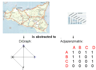
The Digraph-LE is one of four[2] central CAS-LE in this eLA (lasting some hours), where the students should form those skills, which are necessary for a competent successful use of CAS. In the Digraph-LE there is a frame switch to a more static point of view on the concept of matrix as object “[:::]” (figure; table): as context of reference we take a distance table of towns in Sicily/Italy to deepen the concept of matrix and to introduce the corresponding set of elementary matrix operations. Digraphs (i.e. directed graphs), quadratic adjacency matrices and digraph-operations abstract this model situation of a symbolic 'town map' with 4 linked standpoints A, B, C, D allowing different interpretations as bus-, train net, etc.
|
|
|
|
|
Fig. 1: Digraph and associated adjacency matrix M with 0/1 entries to represent ' linked/not linked '. The entry M12=1 is interpreted as 'A is linked to B' and entry M34=0 is interpreted as 'C is not linked to D' |
||
3 Learning elementary programming in the digraph environment
The graphical representation of a digraph (cf. Fig. 1) was given as the CAS-MuPAD black-box plot(diGraph(M)) to the students, because of the use of advanced programming methods. With the aid of this routine the students were able to switch between graphical and matrix representation of a given digraph and to interpret the results of operations on the associated adjacency matrices in the given context.
The adjacency matrix M of the digraph of Fig.1 in MuPAD is noted as
M:=matrix([ [1,1,0,1],[0,0,0,1],[1,1,0,0],[0,0,1,0] ]);
which has the data structure of a list of lists (“row vectors”).
Besides the interpretation of addition, subtraction or multiplication ('folding’) of matrices in this context the interpretation of repeated multiplication Mn:=M*...*M (n times) of the adjacency matrix M of a digraph by itself is especially interesting: the exponent n measures the length (=number of edges) of a path and the (non-reduced-to-0/1 'weighted') matrix entry's itself gives the number of the paths joining two positions. So we distilled the concept of a ”path-matrix” path(M):=SMi (i=1..n, n = number of rows of M), which is a meaningful operation, but hard to calculate by hand (iterated multiplications and additions); the students strongly feel the usefulness of a CAS in this situation.
The path-matrix path(M):=SMi is realized as a MuPAD function, syntactically noted as
path:=(M) -> _plus( M^i $ i=1..linalg::nrows(A)):
Here linalg:: refers to the MuPAD library for Linear Algebra, in which the procedure nrows (=”number of rows”) lives. Now the call path(M); gives back the following result:

Fig. 2: How many paths of arbitrary length go from B to A? The entry path(M)21=2 of the pathmatrix gives the answer; these two prognosted paths are to be seen in the Digraph above: B>D>C>A and B>D>C>A>A (watch the sling!)
So, in contrast to a traditionally CAS free consideration we get a constructive runable concept of a pathmatrix. In the course, this function path() was used in a small project studying a bus net of seven towns, which would not have been so easy without using CAS.
The operations of addition, subtraction and multiplication on adjacency matrices are normally not implemented as build-in routines in a CAS, so we have to write them for ourselves. The problem is, to reduce the result of the normal matrix operation to 0 or 1 in order to retain an adjacency matrix. E.g. two adjacency matrices X and Y are “added” in the following manner: add them as normal and then set every nonzero element to 1. In the modelling example of two transportation nets X and Y the result measures the increase in connection, if the two nets are combined together.
In implementing these operations on adjacency matrices, we use the fact that the programming language of the CAS MuPAD is very flexible and rich. It allows to realize different design plans: here we give a procedural programmed version of the operation of addition of two adjacency matrices
one:=(x)-> (if x=0 then 0 else 1 end_if); // mod 2 possible
ones := A -> (((A[i,j] := one(A[i,j]))
$ i = 1.. linalg::nrows (A)) // $ = for-loop
$ j = 1.. linalg::ncols (A);
return(A));
ADD1 := (A,B) -> ones(A+B);
and here is a functional version, using the predefined library functions zip() and _plus() and the user defined helper function one():
ADD2:=(A,B)->zip(A,B,one@_plus);//f@g=fog=composition
A simple test of these functions looks like this:
A:=matrix([[1,1],[1,0]]); B:=matrix([[0,1],[1,1]]);
ADD1( A,B ); ADD2( A,B );
![]()
The implementation of the other operations is left to our students.
4 Benefits of CAS programming in elementary Linear Algebra
The diGraph-CAS-LU demonstrates the simultaneous introduction and use of mathematical (matrix, operations) and informatic concepts (data and control structure; user-defined vs. built-in functions) in an integrated learning environment. We mention that the process of implementation of the digraph(matrix)-operations in MuPAD seems comparable with Polya's 4-phase problem solving cycle in mathematics, leading in the end to semi- res. fully CAS-automatic calculations. With such simple (semi)automatic MuPAD-functions we can focus on the crucial steps of an algorithm, not getting lost in administrative program-specific technical details. In this way we try to reduce the formal aspect of mathematics res. informatics to the necessary extend and to keep the consideration for our students simple and clear. Also, in the sense of H. Möller (1997) we are able to substitute purely mathematical existence proofs by algorithmically constructions and to support procedural thinking processes.
There is some evidence in our study that the interactive dialogical small group discussion in such an CAS-LU using CAS as an expert system, as knowledge base or as medium to construct wishful automations will support the overcoming of epistemological obstacles in elementary Linear Algebra crucially and stabilize the developed concepts. In transforming the role of the teacher CAS seems to expand the autonomy of the learning process of the students.
References
Baumert, J. e.a. (2000) TIMSS/III - Dritte Internationale Mathematik- und Naturwissenschaftsstudie. Leske+ Budrich, Opladen.
Fletcher, T.J. (1968) A heuristic approach to matrices. Educ. Stud. in Math. 1, 166 - 180.
Laugwitz, D. (1974): Motivations and linear algebra. Educ. Stud. in Math. 5, 243 - 254.
Möller, H. (1997): Algorithmische Lineare Algebra. Vieweg, Braunschweig.
Tall, D. e.a. (2000): The Function Machine as a cognitive root for the Function Concept. PME-NA 22, Bd. 1, 254-261.
Combining CAS with authoring systems
to create flexible learning environments
Csaba Sárvári, Mihály Klincsik and Ildikó Hámori
Pécs, Hungary
2. An algorithm acquirement model supported by CAS and ToolBook
3. Learning model of a complex algorithm
4. Application of the complex algorithm
5. Exercises that require simultaneously handling of many algorithms
Our goal is to show - in connection to a topic of linear algebra - how we can effectively manage the mathematical work and learning, using both a CAS (Maple, in our case) and an authoring system (ToolBook). How does this environment ensure to start from algorithmic primitives and elementary concept building to give step-by-step more work to CAS at allowing to do automatic work at the end.
1 Introduction
The radical regeneration of communication technology, development of computer networks, as well as the appearance of new methods of information storing and info-transmission has caused a didactic paradigm switch. This process was completed in mathematical didactics with appearance of Computer Algebra Systems (CAS). Educators in high schools, colleges and universities can revitalise traditional curricula by introducing problems and exercises that exploit CAS's interactive mathematics. Students can concentrate on important concepts, rather than tedious algebraic manipulations. At the same time involving CAS in the process of teaching mathematics causes a big challenge for didactics.
2 An algorithm acquirement model supported by CAS and ToolBook
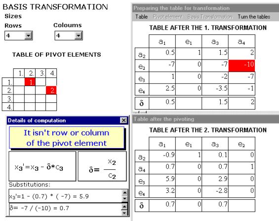
Let us begin with a definition: algorithmic primitive is the most complex activity that the user (a human being or the computer) can understand and carry out directly. In course of the learning and understanding activities the algorithmic primitives are changing, generally they are becoming more complex. As an example, let’s take basis transformation (so-called pivot algorithm), one of the fundamental procedures of linear algebra, which is actually a series of elementary basis transformations.
The steps of the learning process are as follows.
1. Studying and understanding the procedure, with the help of lectures, textbook(s), or subject matters available on the net.
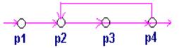
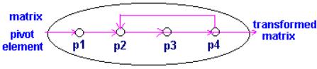
2. As a result of understanding the algorithm, we become able to make out and execute the procedure as a series of the following algorithmic primitives:
Creation of the starting table (P1),
Choosing the pivot element (P2),
Computing the d
-s (P3),
and
Computing the new co-ordinates of the vectors (P4); see Fig. 1.
|
|
|
|
|
Fig. 1: Algorithm built from algorithmic primitives |
||
First, we make execution of the disassembled primitives of the algorithm practised with the help of ToolBook.
|
|
|
|
|
|
Fig. 2 |
|
It has got the following advantages:
it gives the possibility of self-control, while
doing the calculations without computer;
it makes possible to overview and grasp visually
the whole algorithm;
it provides a fine transition to the essentially
automatic computer procedure.
As Fig. 3 illustrates, if the procedure is half-automated, we have access to each step. It means that we can carry out the following interactive steps:
details of the calculation of the new
co-ordinates can be observed;
partial modification and execution of several
versions of the pivot procedure can be followed up.
|
|
|
|
|
|
Fig. 3: The half-automated phase |
|
3. We write the pseudocode of the basis transformation, which could be done in the following form:
procedure elementary (mgen, ngen positive integers, V: matrix)
genel:=V[mgen,ngen] {choosing of pivot-element}
for j:= 1 to coldim (V)
begin
if j¹ngen then {forbidding the column of the pivot-element}
begin
delta:=V[mgen,j]/genel
for i:=1 to rowdim(V)
begin
if i¹mgen then
V[i,j]:=V[i,j]-delta*V[i,ngen]
if i=mgen then V[i,j]:=delta
end
end
end
V[mgen,ngen]:=1
for i:=1 to rowdim(V) {creates the column of the pivot-element}
if i¹mgen then Vfi,ngenG:= 0
V=evalm(V) {it is printed the new matrix}
While writing the pseudocode we have the following didactical goals:
to develop the skill of making an algorithm;
to fix the mental picture of the basis
transformation;
to prepare for writing the Maple procedure.
4. We write the Maple procedure of the elementary basis transformation:
|
|
|
|
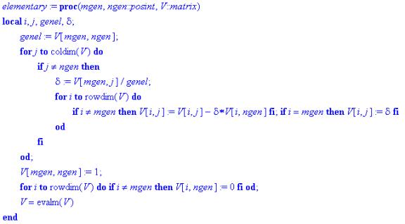
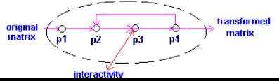
For didactical reasons, we don’t automate the whole pivot algorithm. It would cause an unwanted “black box” effect in teaching of the Simplex method, and it needed too many programming tools. The "elementary" procedure is essentially an automated elemental basis transformation procedure. But it is not a black box, because it is processed step by step with full knowledge of its details (Fig. 4.).
|
|
|
|
|
|
Fig. 4: Schematic picture of the automatic phase |
|
The elliptic outline indicates, that the procedure works automatically with the entered data. We can’t reach the single steps (but it isn’t necessary) any longer.
5. We test the prepared elementary procedure: first we calculate the exercises executed earlier by means of the ToolBook, than we solve further problems using it.
3 Learning model of a complex algorithm
The Simplex method is a complex activity. The successful execution depends on automation of carrying out partial activities. Thus, we can pay attention to survey and build up the whole algorithm. If our exercise is to execute a program that gives the maximum profit, for example, the steps of the learning process are as follows.
We
create the mathematical model from the data: e.g. write the inequalities system
in normal form and the objective function.
To
follow the “traditional” way, we execute the whole algorithm with detailed
calculations. We can make it by using the ToolBook, or we can use the authoring
system only to check the pivot steps.
Half
automated procedure: we use the procedures of the Maple Simplex package
(set-up, feasible, display, ratio, pivoteqn, pivot, cterm). The single
procedures operate as “black boxes”, but the complete procedure is controlled
from outside. We have an overview of the partial steps.
The
automated version means using the "maximize" or "minimize"
procedures of the Maple Simplex package.
As a result of executing the complex algorithm in several way as described above:
we can attain the whole algorithm;
the automated version makes future work faster
and gives possibility of many kinds of generalisations;
The detailed knowledge of the algorithm makes
the user able to go further, to build the knowledge chain further.
4 Application of the complex algorithm
After the above-mentioned preparation the CAS procedures, it is possible to solve such kinds of problems whose solution - because of the time limits or other reasons - wouldn’t be possible in the framework of the “traditional” education. The transportation problem is such an example. Because of the time limit, discussion of this problem in details in the engineering college is not possible. On the other hand using automated procedure, as an illustration and motivation for deeper understanding, we could solve this problem.
|
|
|
|
|
Fig. 5: With help of CAS the Simplex method could be used to solve complex problems |
||
5 Exercises that require simultaneously handling of many algorithms
With help of CAS, we can solve complex, multi-knowledge requiring exercises and problems, which we can’t solve without it. This kind of problem is, for example, the case of minimax polynom (discreet version). In this case we are looking for a polynom of which maximum deviations from reference points are minimal.
|
|
|
|
|
|
Fig. 6 |
|
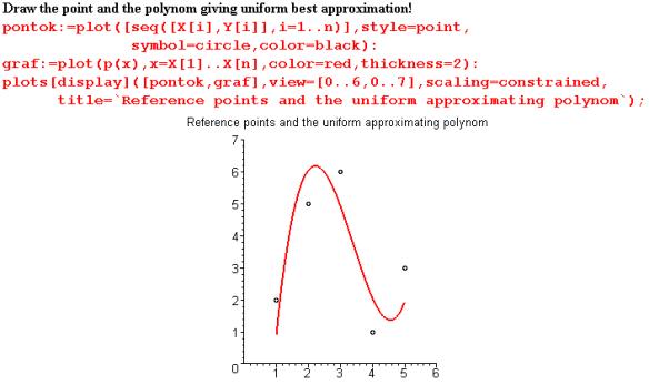
We can compare the obtained approach with the Taylor polynom approximation. If the degree is one less than the number of points then we get interpolation (Fig. 7).
|
Fig. 7: Solving complex problems contributes to the densification of the knowledge-representation net |
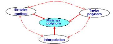
We consider the above-mentioned model to be important because the points of
creating knowledge-representation net and
enriching it in connections;
making connection between discrete (simplex
method) and continuous systems (Taylor).
6 Summary
By means of ToolBook authoring system and CAS (Maple) together we can make such a learning environment, which is able to enforce the characteristics of mathematical recognition of CAS, while we can avoid the damage of versatile, circumspect concept building. Simultaneously, we direct the process of learning so that the knowledge-representation net becomes adequate density. We can build active connections between the different chapters of Mathematics, this way enhancing the building up of transfer. This leads to applicable mathematical knowledge.
The paper shows that CAS may be integrated into teaching of Mathematics in a way, that
the concept building becomes multi-faceted,
combining analytical, graphical and numerical approaches, where it is possible;
the “black box” effect in the concept building
is avoided;
substantial questions are of primary interest;
we are expecting didactic and professional surplus value from application of CAS.
References
Ambrus, A. (2000) Standpunktwechsel beim Problemlösen. Beiträge zum Mathematikunterricht 2000, 77-80.
Mérő, L. (1997) Észjárások. Tericum Kiadó. Budapest
Dobi, J. (1998) Megtanult és megértett matematikatudás. Az iskolai tudás. Osiris Kiadó, Budapest, 169-188.
Greeno, J.G. (1977) Process of understanding in problem solving. Castellan, N.J., Pisoni, D.B. and Potts, G.R.: Cognitive theory. Lawrence Erlbaum, Hillsdalle, NJ. Vol. 2, 43-83.
Popper, K. (1994) Knowledge and Body-Mind Problem. Routledge, London.
Johnson-Laird, P.N. (1983) Mental Models. Cambridge University Press.
[1] Fletcher (1968, 167) wrote: “But at the same time the problem must not seem trivial, and there must be room for experiment, for different strategies and preferably for more than.
[2] The other CAS-LE are a visualization of Gauss-Algorithm (presented also as CAS-game; inclusive concept of inverse matrix), under-determined linear systems and the concept of orthogonality (via looking at the solution sets of homogeneous linear systems) and over-determined LS and the concept of pseudoinverse (for the solution of regression problems).