Special Group 3:

Hand-held technology

Jan Kaspar and Alison Clark-Jeavons

Prague, Czech Republic, Littlehampton, UK

Piotr Bialas	Anova with the TI-83 graphing calculator
Piotr Bialas	Linking graphing calculators to the Internet
Jan Kaspar	Programming as a tool for the precision
Regis Ockerman	Probability simulations with TI 83(p)
Jarmila Robová	Graphic solutions of equations and their systems

1. The group

2. Hand-held technology

3. The hand-held technology demonstrated

1 The group

Four authors submitted between them five contributions, all of which were presented. Attendance at presentation varied between 8 – 10, all were followed by a discussion. All contributions were based on graphing calculator TI-83. Considering that many other special groups and working groups also attended contributions relevant to hand-held technology (mostly its applications), it raises a question, whether a “special” hand-held group will be necessary in the future.

2 Hand-held technology

This term encompasses the technology of graphing calculators, notebook and palm-top computers, the key features of which combine calculator and computer technology. The facilities offered by each type will vary from model to model. Essentially they all offer built-in software and functions, which allow for the exploration of mathematical concepts. Some hand-held technology will offer symbolic manipulation and most will enable data to be transferred and exchanged.

3 The hand-held technology demonstrated

All presenters in this special group chose the Texas Instruments TI 83 Graphing Calculator and Viewscreen as hand-held technology for their activities.

Pjotr Bjalas, USA: Linking graphing calculators on the Internet (LGCI)

Pjotr demonstrates how the data can be transferred between PC and graphing calculators (esp. the TI-83), how LGCI increases addresses to the data files, avoids the burden to type data into the graphing calculator and how it makes possible that the selected data files may be used for Excel, Minitab, SPSS and many other statistical software products. In the discussion, there was a dispute about the size of data files transferred.

Regis Ockerman, Belgium: Probability simulation with the TI-83

Regis demonstrates, how it is easy to do simulations, dealing with problems of probability, taking advantage of the possibilities of the TI-83. In his presentation of workshop type, he simulated the real work in class, which was very appreciated by the participants.

Jarmila Robova, Czech Republic: Graphing solutions of equations and their systems

Jarmila presented several techniques of graphic solution of equations and their systems: Geometric representation of problems, solution using Boolean algebra, graphic solution, using the graphing calculator TI-83. In the discussion, she spoke about experience from seminars at Charles University in Prague.

Pjotr Bjalas, USA: Anova with the TI-83 graphing calculator

In this contribution, Pjotr demonstrates, how the Catalog and Cut-and-Paste utilities of the TI-83 graphing calculator may be used to complete one-factor Anova tables. This presentation was a workshop, where worksheets including two examples, were distributed. He demonstrated that an extension may include two-factor Anova such as 2x2, 2x3 or 3x3 factorial design.

Jan Kaspar, Czech Republic: Programming as a tool for precision

Using very simple examples, Jan demonstrates, how programming requires precision in the step-by-step description of the mathematical tasks involved. He demonstrates that erroneous results of some programs may directly be referred to mistakes in the step-by-step description of the algorithms being used. In the discussion, all participants, with experience of seminars for students – prospective teachers of mathematics, agreed, that most of the difficulties arise in the accurate description of the simplest calculation procedures.

Goto
	Begin of article		Contributions by authors
	Begin of session		Main page

Anova with the TI-83 graphing calculator

Piotr Bialas

New York, USA

1. Example

2. Solution with the TI - 83

3. Outline for the Anova procedure

4. One-way Anova calculations with the TI-83

5. Anova table with the results

This paper will demonstrate how Catalog and cut-and-paste utilities of the TI-83/TI-83 Plus graphing calculator can be used to complete a one-factor Anova table. Extensions may include a two-factor Anova such as 2x2, 2x3, or 3x3 factorial designs. The author believes that this not very technical illustration of Anova method allows students with a limited statistical background for efficient application of it and perhaps helps them in better understanding of the inner workings of the Anova methodology.

1 Example

Compare the cleansing action of three detergents on the basis of the following whiteness readings made on 15 swatches of white cotton cloth, first soiled with organic oil and then washed in an agitator-type washing machine.

Detergent A	Detergent B	Detergent C
154	144	152
162	116	170
142	148	164
152	132	160
160	140	154

2 Solution with the TI - 83

Suppose all theoretical assumptions related to sampling, distribution of whiteness readings, and error distribution are met.

Suppose that the variance of readings for each detergent is approximately the same.

Method: One-Way Anova – Model: FIT + RESIDUAL = DATA

3 Outline for the Anova procedure

Set up the hypothesis
Transfer the data to the TI-83 graphing calculator into List Editor of STAT menu.
Use the variance among the lists’ means to estimate the variance of the 15 whiteness readings, (by the Central Limit Theorem: s ^2 = s ^2mean· n, where n is the number of elements in the sample). This quantity is the MSE between entry in the Anova table.
Pool the respected variances of L1, L2, and L3. This quantity is the MSE within entry in the Anova table.
Calculate the F observed :	F observed =
Calculate the p-value:	p-value = 1 – Fcdf (0, F observed, df between, df within)
Conclude about H0

4 One-way Anova calculations with the TI-83

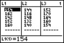
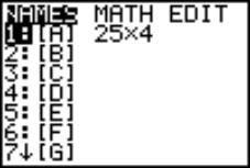
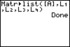
The following screen displays of the TI-83 graphing calculator will correspond to the three parts of typical one-way Anova table: Between, Within, and Total part. The data was entered in the list format into the TI-83 graphing calculator. It was initially saved in ASCII format on my desktop and then transferred with TI GRAPH LINK (83) to my TI-83 graphing calculator, no typing was required, see Fig. 1.
	Fig. 1
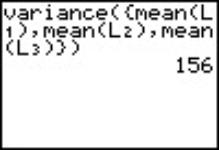
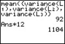
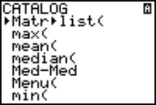
Hypothesis H0: The means of the lists are equal. Ha: The means of the lists are not equal. Between part of calculations involves estimate of variance based on lists L1, L2, and L3. The Catalog utility in the TI-83 was used in order to access and concatenate respective commands, see Fig. 2.
	Fig. 2
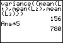
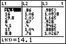
Mean Squared Error of variance among all measurements will be calculated, see Fig. 3. The MSE between quantity calculation was based on the Central Limit Theorem. MSE between = 780
	Fig. 3
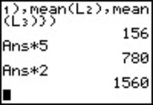
The last part of Between involves the estimation of the sum of squared deviations, Fig 4. The sum of squared deviations was calculated as a product of MSE between and df between
	Fig. 4
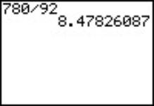
Within part of calculation will involve variance for each list. The MSE within quantity was calculated by “pooling” the three variances. The sum of squared deviations was calculated as a product of MSE within and df within. The F observed quantity will be calculated in order to determine the p-value and make a decision with respect to null hypothesis, see Fig. 6 and 7.
	Fig. 5
Fig 6	Fig. 7: Conclusion with respect to H0
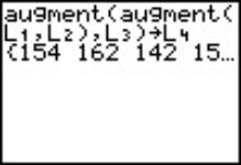
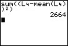
Total part of calculations of this Anova table will involve computing of the sum of squared deviations, see Fig. 8-10. The list L1 was augmented by L2. The resulting list in turn was augmented again by L3 and saved as L4
	Fig. 8
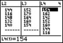
The total sum of squared deviations from the Grand Mean was calculated. The obtained results were summarized in the table below.
	Fig. 9
	Fig. 10

5 Anova table with the results

Source of Variation	Df	Sum of Squared Deviations (errors)	MSE	Fobserved	p-value
Variation Among Means of Lists Between	2	1560	780 Estimated population variance	8.4783	.0051
Variation within Lists Residual or error variation Within	12	1104	92 “pooled” variance
Total	14	2664

References

Freund, J., Simon, G. (1997). Modern Elementary Statistics. Prentice Hall, New Jersey.

Goto
	Begin of article		Contributions by authors
	Begin of session		Main page

Linking graphing calculators to the Internet

Piotr Bialas

New York, USA

1. Introduction

2. Linking the graphing calculator to the Internet

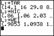
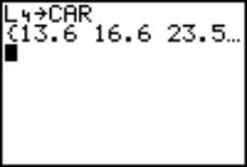
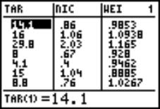
Linking graphing calculators to the Internet (LGCI) increases access to the numerical data files, provides no need to type the data into the graphing calculator, and makes possible, that the selected data files may be used for Excel, Minitab, SPSS, and many other statistical software products. The TI-83 example of the data transfer will be demonstrated.

1 Introduction

Information about the file downloaded from the Internet

http://www.amstat.org/publications/jse/v2n1/datasets.mcintyre.html

Name: Cigarette data for an introduction to multiple regression

Type: A sample of 25 brands of cigarettes

Size: 25 observations, 5 variables

Descriptive abstract

Measurements of weight and tar, nicotine, and carbon monoxide content are given for 25 brands of domestic cigarettes.

Sources

Mendenhall, William, and Sincich, Terry (1992), _Statistics for Engineering and the Sciences_ (3rd ed.), New York: Dellen Publishing Co. (ISBN: 0 02380552 8; Original source: Federal Trade Commission, USA)

Variable descriptions

Brand name

Tar content (mg)

Nicotine content (mg)

Weight (g)

Carbon monoxide content (mg)

Values are delimited by blanks. There are no missing values.

Story behind the data

The Federal Trade Commission annually rates varieties of domestic cigarettes according to their tar, nicotine, and carbon monoxide content. The United States Surgeon General considers each of these substances hazardous to a smoker's health. Past studies have shown that increases in the tar and nicotine content of a cigarette are accompanied by an increase in the carbon monoxide emitted from the cigarette smoke. The data presented here are taken from Mendenhall and Sincich (1992) and are a subset of the data produced by the Federal Trade Commission. For more information, see the article "Using Cigarette Data for an Introduction to Multiple Regression" by Lauren McIntyre in Volume 2, Number 1, of the Journal of Statistics Education.

2 Linking the graphing calculator to the Internet

Question 1

Why does linking the graphing calculator to the Internet make sense?

Answers

Increases access to the numerical data files

Provides no need to type the data into the graphing calculator

Makes possible that the selected data files may be used for Excel, Minitab, SPSS, and many other statistical application software products

Provides incredible time savings

Does not tie up to the specific TI graphing calculator

Motivates student research on the Internet

Allows advanced beginner student to do independent projects

Question 2

What accessories do I need to transfer a numerical data from the Internet to the TI-83 graphing calculator?

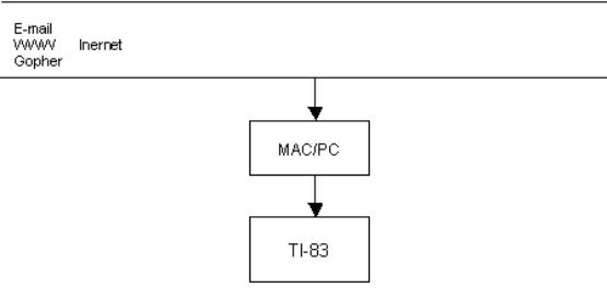
Answer: I need TI-Graph Link for the TI-83 graphing calculator, (communication software installed on my HD), and linking cables, different for Mac and PC, see Fig. 1.

Fig. 1

Question 3

How do I transfer a numerical data file from the Internet to the TI-83 graphing calculator?

Answer: Change selected Internet files format into the TI-83 matrix/list format, see Fig. 2.

Fig. 2

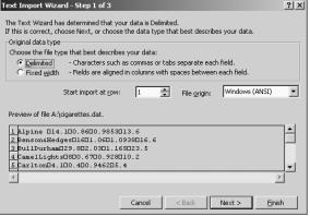
Question 4

How do I change the selected Internet numerical file into the TI-83 matrix/list format?

Answer: First, open the selected Internet file with a spreadsheet program, (e.g. Excel), and beautify it. Second, select the numerical data, and copy that to the Graph-Link software. Third, save the selection in ASCII format. Fourth, use Tools menu and select Import ASCII Data option, in order to open previously saved data. Last, save the file in the TI-83 matrix/list format, see Fig. 3.

Fig. 3

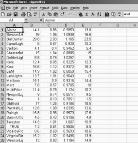
See Fig. 4 and 5 below.

Fig. 4

Fig. 5

Goto
	Begin of article		Contributions by authors
	Begin of session		Main page

Programming as a tool for the precision

Jan Kaspar

Prague, Czech Republic

1. Introduction

2. Examples

3. Short résumé

Using the TI-83 graphing calculator I would like to demonstrate how programming requires precision in step-by-step description of mathematics tasks.

1 Introduction

In teaching mathematics we often find that although the students can solve mathematical problems, they cannot adequately describe their solution process step-by-step. I think that programming can help to deal with this problem. If there is need to construct an algorithm for a particular solution process, this process must be described step-by-step in programming. In view of the fact that newer hand-held technology is equipped with a programming language that makes use of principles of structural programming, they would be a useful tool for tackling this problem. In this brief contribution I would like to demonstrate on some very simple problems how their algorithmisation automatically forces the author of the program to describe the solution steps accurately. For all of the following examples the graphing calculator TI-83 has been used. For those not familiar with this particular model, let me just mention that its programming language has, in addition to the usual “input-output” procedures, the following basic statements (among others):

the conditional test “If Then Else”

the incrementing loop “For”

the conditional loops “While” and “Repeat”

the end of a block signification “End”

a program as a subroutine execution “prgm”

(and only “one-letter” identifiers - name of variables, are available).

2 Examples

Four very simple examples – programs are introduced for the purpose of demonstration. For each of them detailed commentary is given concerning those commands, where accurate formulation in the description of the relevant calculation algorithm is essential. Such accurate commands are necessary preconditions for the generated program to perform the calculation of a given problem correctly.

Example 1

Write a program for solution of equation a*x² + b*x + c = 0. Let me offer you my solution with comments.

PROGRAM:QE :Real :ClrHome :Prompt A,B,C	These 3 statements illustrate, that we’ll work in real mode, start with a clear display, and 3 values of coefficients a,b,c are asked (their values are necessary, when we start the solution process)
:Fix 2	The statement for results‘ edition (2 decimal)
:If abs(A) < 10^(-6) :Then If abs(B) < 10^(-6) :Then If abs(C) < 10^(-6) :Then :Output(5,1,”ALL X”) :Else	Very important part of program. We have to discuss all possibilities of the coefficients (a,b,c) values and have to finish solution in each of branch. As a “side effect” in this discussion is test, if a value of each of coefficients (a,b,c) = 0. Because they are stored as real variables in the calculator, it is not a good idea to use a “direct” test (If “v=0”). For real variables is better to test, “ if variable Î or Ï of e- neighbourhood of 0”.
:Output(5,1,”NO X”) :End :Else :-C/B->X :Disp X :End :Else :B^2-4*A*C->D
:If D<0	The complex mode is necessary if D<0.
:Then :a+bi :End
:(-B-Ö(D))/2/A->X	Very important statement in this form; it illustrates that equal priority of operations must be respected.
:(-B+Ö(D))/(2*A)->Y :Disp X :Disp Y :Stop	And in this statement there is illustrated how the brackets influate priority of operations and help us to use for formulas “pretty” notation.

Example 2

There is shown, in two following examples, how it is useful to choose “more convenient” of two conditional loops with different philosophy:

“while” loop – at first the condition is tested; if “true”, all statements inside loop are executed and the loop is repeated, if “false”, no statement inside loop is executed and the following statement after “while” loop is executed

or

“repeat” loop – statements inside loop are executed and when the execution of these statements is finished, the condition is tested; if “true”, “loop” is finished and the following statement after “repeat” loop is executed, if “false”, loop is repeated.

This moment is very important indicator, if we understand what we wish to do, what we wish to achieve.

Problem 2.1

Two integers A and B are given. Use the Euclid algorithm to evaluate the greatest common divisor. The program is very simple, of course.

: PROGRAM:  NSD :Prompt A, B :While A¹B :If A>B :Then :A-B->A :Else :B-A->B :End :End :Disp A:Stop

In this case it is better to use “while” loop, because if values of given A and B are equal, we haven’t to do anything, “while” loop give us result directly. Sometimes, if “repeat” loop is used, when it is not convenient, one “back-step” it is necessary to provide.

Problem 2.2

For “Repeat” loop let me offer this helpful example: Evaluate the sum of the series S (1/2)ⁿ (n = 0, 1 … ) with given accuracy e. The program is very easy, again:

:PROGRAM: SUM :Prompt E :0->S :0->N :1->D :Repeat D£E :N+1->N :(1/2)^N->D :S+D->S :End :Disp S:Stop

It’s clear in this example, that we have to go through the block statements inside “repeat” loop at least once, to obtain required accuracy.

There is another very important moment. It isn’t necessary to evaluate in each step (1/2)^2, (1/2)^3 etc. When we can evaluate (1/2)ⁱ it is better to compute it as (1/2)^i-1 * (1/2); in the program we cancel the statements:0->N and:N+1->N and the 5^th line we substitute by statement :1/2*D->D)

In the last example I would like to illustrate, how it is helpful for description (and understanding) of solution of large, complicated problem, if that solution is split into several solutions of partial, simple problems.

Example 3

The line p and two different points A, B in the same half-plane are given, none of which lies on the line p. Find such a point P on the line p, that the sum of lengths of segments AP and BP is minimal.

Solution: What we have to do, when we solve this example “with pencil and paper”:

we have to find an image point A’ of the point A in symmetry with respect the line p

we have to draw line q, passing though points A‘ and B

we have to find the result point P as intersection of p and q

But the first step isn’t elementary; there are three steps inside, in fact:

we have to draw perpendicular line k to line p passing through point A.

we have to find intersection of p and k – point Q.

we have to find point A’ on line k, in opposite half-plane than point A is, to be AQ and A’Q equal segments.

Now, when the example is analysed, we can start to write program or subprograms for each elementary step. Let me suppose, we solve this example in plane, so that a point has two coordinates x and y and a line is described by general equation a*x+b*y+c = 0. There is very easy solution for this (and similar) situation:

Let me suppose that we have written the following subprograms for “input point” and “input line”:

prgm RP – input of point (two coordinates)

prgm RL – input of line (three coefficients of general equation)

the subprograms for partial, simple calculation:
prgm PLP – subprogram returns three coefficients of equation of line, perpendicular to given line (by three coef. of eq.) and passing through given point (by two coord.)
prgm PPL – subprogram returns three coefficients of equation of line, passing through two given points (by two coord.)
prgm LLP – subprogram returns two coordinates of point, intersection of two given lines (by three coef. of eq.)

The last subprogram for the construction of the point A’ symmetric point with given point A with respect to the line p is missing. This problem we can solve, using vectors (vector AA’ = 2* vector AQ). It’s useful to write subprogram not for “2*vector” but for “n*vector” and use n = 2. Let us assume that we have written such a subprogram

prgm NV – subprogram returns two coordinates of end point E’ of vector AE’ = n*vector AB where A is starting point of both vectors and B is end point of given vector

And now we can write very easily the final program, it is sequence of subprograms:

:prgm RP:prgm RP :prgm RL :prgm PLP :prgm LLP :prgm NV (for n=2) :prgm PPL :prgm PLP

In fact, the solution of “large, complicated” problem is described very precisely by solution of partial, simple problems.

And having these subprograms (solution of partial, simple problems), we can describe precisely solution of a lot of other problems (triangle’s midpoint or centroid, etc., etc).

3 Short résumé

An important indication of the need to improve the description of a mathematical procedure is to find that the program leads to incorrect results. In such a case it is quite likely that step-by-step description used in programming has not been correct.

Goto
	Begin of article		Contributions by authors
	Begin of session		Main page

Probability Simulations with the TI 83(p)

Regis Ockerman

Stekene, Belgium

1. Introduction

2. Distribution of the results when throwing a die

3. First problem of Chevalier de Méré

4. Second problem of Chevalier de Méré

5. At least two equal results when throwing four dice

1 Introduction

Two years ago, in the Dutch speaking part of Belgium the curriculum changed for mathematics in secondary schools. In 3^rd and 4^th year working with graphics and statistics was introduced, including elementary probability. Also teachers had to reserve at least 20% of the time for the use of ICT, in a way that students will be able to use it on their own. This implicated that students need their own personal calculator. Taking account of necessities and price, a lot of Ti 83 where introduced (individually or offered in a loan - system from the schools). For doing statistics, The TI 83 provides powerful functions for the use of lists. Also provided is a random function, which gives the possibility of simulating probability. Two of my colleagues of T3-Flanders, Guido Herweyers and Koen Stulens wrote a book on statistics, taking advantage of a graphing calculator.

In agreement with my colleagues, apart from some introduction, I will not deal with problems elaborated in the book, such as: the birthday-problem, the switching of hats…

2 Distribution of the results when throwing a die

As well known, the possible results are the integers from 1 to 6, each of them with equal possibility, so the probability for each result is 1/6.Simulating the throw of a dice can be done with the function randInt(1,6) that returns an integer from 1 to 6. Pushing again on the enter button, we get a new number and so we get an impression of throwing several times. We can do this at once by entering a third number in the function like randInt(1,6,4), which indicates that we throw a die four times. Normally it is more convenient to store this sequence in a list and then we get randInt(1,6,4)üL�.

Theoretically, when we use the expression randInt(1,6,60)üL�,we could expect for each number a frequency of 10; but we know that this is only so for large numbers.

In class, we can collect a larger number of data if we let each student do this simulation. We have to give each student another seed value, which determinates the sequence of produced random numbers. Default the seed value is 0, but can be changed by the expression e.g. 10àrand, which puts the seed value on 10. In class it is easy for students to take their “classnumber“ as random seed number. This must be done before using an expression with randInt.

We can easily analyse the frequency of the numbers in the sequence by taking advantage of the graphic possibilities of the calculator and put them in a histogram. By tracing this plot, we can easily notice the frequencies and then collect them. To do this in an elegant way, we use a program: DICE1

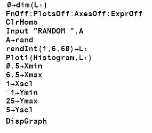
Suppose a class with 20 pupils. The teacher can collect the data of each student and put them in the Lists L1 to L6 . Making the sum of the lists gives an idea of the frequency distribution. This example is used in many course books.

3 First problem of Chevalier de Méré

For those who are not familiar with it, the formulation is: “What’s the probability to have at least one 6 when throwing a dice four times?”

This is a good example, which shows that it is sometimes better to use the complement. So we obtain 1 – (5/6) ⁴ = 0.5177469136. For convenience, we use a program. We store the results of four throws in a list and check if one of the elements is a 6, which results in the program DI46 In this program we will take advantage of some powerful built-in functions of the TI 83. Let us put the numbers 1, 6, 4 and 2 in the list L�. The expression L�=6 is a logic evaluation and returns a sequence of 0 and 1, the 1 on the places where we have a 6 in the sequence L�. Also we can make the sum of the 1’s in the sequence. This can also be used in logic equation. So, searching if there is at least one 6 in the sequence means that the evaluation sum(L1=6)>0 must be true (returning 1).

We hope to have 20 participants, so we can collect a large amount of data. Using the emulation program VTI on a Pentium III 667, I collected data from 10 000 simulations and the result was 0.5215, which matches closely the theoretical value.

4 Second problem of Chevalier de Méré

What is the probability of having at least one 66 when throwing 24 times with two dice? Again this is easy to calculate, using the complement: 1 – (35/36) ²⁴ = 0.4914038761. We use the program DI22466

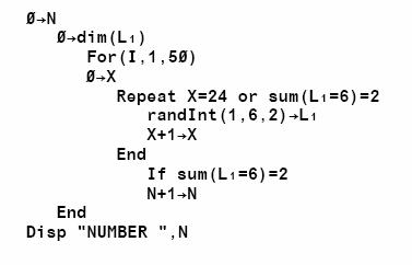
Since, in a worst case situation, we have to throw the dices 24 times; it’s convenient to use the repeat until instruction, so that we can jump out if the condition L�(1)=6 and L�(2)=6 is satisfied, expressed as sum(L�=6)=2. This program is very demanding and takes a lot of running time. Since the probability is very close to 0.5, we need a large amount of data. Again, I based my conclusions on 10 000 simulations and obtained 0.4848, very satisfying for me.

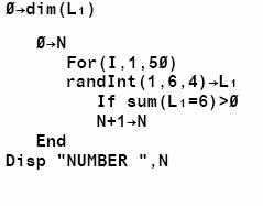
5 At least two equal results when throwing four dice

Once again, this can easily be done with the complement, which can be described as: the four results must be different. This leads to the probability: 1-(6*5*4*3/6^4)= 0.72222

In the program, we use some powerful instructions of the TI 83. First of all, we can sort a list. Then we can calculate the differences. If two elements are equal we will get 0 in the list of the differences. When all the components of a list are different, we get sum(¾List(L�)=0)=0. We use the program DI4AL2E

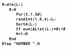
Collecting data from over 12 000 simulations, I got the result 0.720988.

The content of this contribution can be used freely for educational purposes. This is only a short version. The total version will be on CD. If you want it already now or if you want dumps of the programs, which can be used directly with the TI-Graph Link, just contact me via e-mail.

Acknowledgements: I wish to thank all the participants for their engagement and co-operation. I am very grateful to my chairs: Alison Clark - Jeavons and Jan Kaspar, for their support. My special thanks to Per Broman for his useful suggestions.

References

Herweyers, G. and Stulens Koen Statistiek met een grafisch rekentoestel. Acco, Leuven.

Grabinger, B. Stochastik mit Derive. Duemmler, Bonn.

Kutzler, B. Improving Mathematics Teaching with Derive. Chartwell-Bratt.

Adler, I. (1963) Probability and Statistics for Everyman. John Day, New York. (In Dutch: Waarschijnlijkheidsrekening en Statistiek. Aula.)

Texas Instruments Guidebooks for TI-83 and TI-83 Plus.

Goto
	Begin of article		Contributions by authors
	Begin of session		Main page

Graphic solutions of equations

and their systems

Jarmila Robová

Prague, Czech Republic

1. Solving equations and inequalities graphically

2. Solving equations using Boolean functions

3. Solving equations by algorithm, formula

4. Connecting of techniques

5. Conclusion

The solutions of equations and their systems belong to basic skills that students acquire in algebra course in the secondary school. In traditional mathematics teaching the students learn how to simplify terms in equations and how to manipulate algebraic expressions using equality properties, factoring polynomials etc. In general, students learn to solve equations by performing operations that produce simpler equivalent equations. Students spend much time by learning these algorithms and procedures, however, often without understanding of meaning and connections. This often results in students’ having isolated knowledge and in their making little or no connections to the related areas of mathematics. Graphic calculator allows students and teachers to apply new procedures of solution processes. The solutions of mathematical problems by different techniques and ways contribute to better understanding particular parts of mathematics, their mutual interconnecting. In the following parts these ideas are illustrated by several examples.

1 Solving equations and inequalities graphically

It is self-evident to students that it is helpful to use the graphic methods of solutions. They easily draw graphs of the functions, which occur in the equations, and then they determine the zeros or intersections as required by the character of the equation form. The significance of this solution technique can be seen in several aspects. Firstly, the graphic representation of problem leads to creating of correct images of the mathematics objects and relationships between them. For instance, the equations with parameters belong to difficult types of equations for students because they must learn the difference between parameter and variable. Graphical methods can help in this respect.

Example 1: Determine the number of solutions for the equation x + ½p‑x½ = 3 with variable x Î R and parameter p Î R.

Traditional paper-and-pencil method is more nerveless than graphic solution. We draw the graph of the function on the left side for several values of p (p = -2, 0, 1, 4) and the graph of constant function from right side of equation (Fig. 1). Comparing mutual positions of graphs we determine that for p = 3 infinitely many solutions exist, for p < 3 just one solution exists (for p > 3 the solution set is empty).

Fig. 1

Secondly, the graphic methods of solution mediate the relationship between algebra and geometry. Depending on the type of equations (linear or quadratic) we can investigate the mutual position of two lines by comparing their slopes and y-intercepts, we can explore common points of conic section and line or the mutual position of two conic sections (Robová 2001a).

Further, the graphic techniques of equations solving can also help in traditional procedure - paper and pencil method - as a tool for the control and/or estimation of the solution. Especially, when we solve the equation or inequality using non-equivalent operations (for example squaring) we can get some “extraneous solutions“, which are not solutions of the original equation or inequality. Therefore we check all the solutions by substituting them into the original formula and eliminate the extraneous solutions. In the case of radical inequality with infinitely many solutions, they cannot use this technique. There is impossible to substitute all the solutions to the original equation or inequality. However, we can apply graphic method to check the solution set.

Example 2: Solve the inequality Ö(5-x) > x+1.

Paper-and-pencil method: Conditions: x £ 5 (radical) Ù x ³ ‑1 (to make squaring the equivalent operation)

Squaring: 5-x > x² + 2x + 1 …

0 > (x + 4).(x - 1)

Conclusion: x Π(‑4, 1) Ç conditions leads to the wrong solution: x Π[‑1, 1). Most of the students obtain this wrong incomplete solution because they forget that the inequality is true for all x, where x + 1 < 0.

Right solution: x Π(‑¥, -1) È [-1, 1) Û x Î (‑¥, 1)

Graphic solution: We can use the graphic calculator to solve the inequality and write both functions to editor as y = Ö(5‑x) and y = x+1, then we graph these functions and compute their intersection point (Fig. 2). For better imagination, we can shade the area above and below the graphs (Fig. 3). Then we can read the right solution directly from the display.

Fig. 2	Fig. 3

2 Solving equations using Boolean functions

Boolean functions are not often used techniques. Nevertheless, this technique contributes to understand the linkage between propositional functions and equations or inequalities. The students may better take in the proper meaning of what to solve an equation or an inequality means if the problem is reformulated to the task to find the truth set of the propositional form.

Example 3: Solve this equation x - ½x + 4½= 2x + 4 .

We enter the expressions from both sides of the equation to editor as Y₁, Y₂ and write to editor the "Boolean function" Y₃ = (Y₁ = Y₂), see Fig. 4. The function Y₃ has the range {1, 0} - it means that Y₃ = 1 for Y₁ = Y₂ and Y₃ = 0 for Y₁ ¹ Y₂ - and draw the graphs (Fig. 5). The solution set is the interval (-¥, -4].

Fig. 4	Fig. 5

3 Solving equations by algorithm, formula

Due to programming possibilities of graphic calculators it isn’t difficult to create and use a program for the solution of some equations (Robová 2001b). This approach is particularly suitable when the graphic solution is not realizable. For instance, for a quadratic equation with discriminant less than zero, the graph has no zero points.

Example 4: Find the solutions in the field of complex numbers 4x² ‑ 16x + 17 = 0.

We set up complex number in menu, then we store the value 4 to variable A, -16 to B and 17 to C. Now, we write the known formula for the roots of quadratic equation on home screen (Fig. 6) by using the list {-1, 1} for the sign " ± and obtain the complex roots (Fig. 7).

Fig. 6	Fig. 7

4 Connecting of techniques

While using graphic calculators in mathematics teaching, we don’t use mentioned techniques separately one from another, but in mutual interaction. The students usually use the graphic method first and they often interpret used procedure in a geometric way. If the students meet some difficulties during graphic solution and graphic method doesn’t yield the desired solution, then they choose another technique like a Boolean function, an algorithm and so on.

Example 5: Solve the equation 3x² ‑ 10x ‑ 8  =  0.

We proceed by a customary way – firstly we draw the graph of quadratic function on display, then we find the solutions using command zero (Fig. 8 and 9). One of the solution (Fig. 8) looks like the rational number with a one-digit period.

Fig. 8	Fig. 9

We use the second precise root and Viete’s formula for the relation between coefficients and roots x₁, x₂ of quadratic equation x² + px + q  =   0 (x₁ + x₂ = ‑p  Ù x₁ x₂ = q). For our equation, p = ‑¹⁰/₃ and q = -⁸/₃. We know the root x = 4, therefore the second root is -²/₃.

5 Conclusion

There are many conditions in educational process determining how we teach and how the students learn. Graphic calculators and their use in mathematics teaching can help to create positive attitudes toward mathematics and make mathematics alive and interesting for the students while they learn. Consequently, graphic calculators can assist to improve mathematics teaching and to enhance the students’ skills and knowledge. Multiple-representations of mathematics problems, e.g. the solutions of equations, by using graphic calculators enable to link particular parts of mathematics - algebra with geometry, algebra with propositional calculus, algebra with function theory.

References

Demana, F., Waits, B. K., Clemens, S. R. (1994) Precalculus Mathematics. A Graphing Approach. Addison-Wesley.

Robová, J.(2001a) Geometric problems and graphic calculator. Mathematics-Physics-Informatics 10, 307-312.

Robová, J. (2001b) Using TI-83 in Algebra in Czech Republic. Proc. T³ Int. Conf., Dallas 2001, CD

Goto
	Begin of article		Contributions by authors
	Begin of session		Main page