Special Group 1:
Derive, TI-89/92 and other CAS
Josef Böhm, Bernhard Kutzler and Marlene Torres-Skoumal
Würmla, Hagenberg, and Vienna, Austria
|
How to make tests for students that are using a CAS tool (TI-89) |
|
|
Issues on integrating CAS in teaching mathematics: A functional and programming approach |
|
|
Animiertes Grafiken-Zusammenspiel von PC und TC in der Mathematik |
|
|
From pole to pole — A numerical journey to an analytical destination |
|
|
Fermat’s Little Theorem: A thing of beauty is a joy for ever |
|
|
Elimination of parameters and substitution with computer algebra |
|
|
Theorema-based TI-92 simulator for exploratory learning |
|
|
Krümmung als Grenzwert — Curvature as limit |
|
|
Mathematics with graphic and symbolic calculators — Teacher training in Lower Saxony |
|
|
Standardizing the normal probability distribution — An anachronism?! |
|
|
Using a CAS to teach algebra — Going beyond the manipulations |
|
|
Introducing Fourier Series with Derive |
|
|
The TI-89/92 as a tool for analytic geometry |
|
|
The use of CAS in the Thuringian school system: Present and future |
|
|
Computers and Computer Algebra Systems in engineering education |
|
|
Ortskurven — Loci |
|
|
Advantages and dangers in the teaching of stochastics by using CAS |
1. History of this special group
3. Categorising the contributions
4. Benefits and prospects of the working group
1 History of this special group
I was very honoured to receive an invitation to chair a special group "CAS" at the occasion of the ICTMT 5. Then I found in the conference program another special group "Derive and TI-89/92" chaired by my friends Vlasta Kokol-Voljc from Maribor, Slovenia, and Bernhard Kutzler from Hagenberg, Austria. As we all found it useful to join our two groups we asked the organizers for doing so and they agreed.
We used our email address books to invite colleagues and friends from all over the world to contribute for the ICTMT 5 in general and for our special group specially. At the beginning we had only a few submissions. Our very reliable CAS – friend Carl Leinbach from Gettysburg College, USA, was the first to submit a paper. And from one day to the other we had more and more contributions in our mailboxes. Finally we found that we had gathered the largest special group of all around us and we had to ask the organizers for some additional slots in the timetable.
Immediately before the conference we had 20 lectures planned. Two people had to cancel – Ernö Scheiber from Romania and Mykola Kolodnytsky from Ukraine, so 18 lectures remained. Vlasta and Bernhard did a good job preparing the schedule and my job was to urge the group members for sending the abstracts and papers in time.
I am very grateful that all our participants were very reliable and dutiful and delivered their lectures without exceeding the deadline.
Some weeks before the conference Vlasta had to cancel her presence at Klagenfurt because of personal reasons and we were very grateful that Marlene Torres-Skoumal from the Vienna International School took her job. Bernhard, Marlene and I agreed that each of us should chair the group one day, and so we did.
2 At the conference
We had 18 submitted and accepted papers. The colleagues came from 8 different countries:
USA 1, Germany 6, Belgium 1, Netherlands 1, Sweden 2, Ireland 1, Turkey 1 and Austria 5.
Two of the submitters applied for giving a workshop: Alex Lobregt from the Netherlands wanted to show how to "Introduce Fourier Series with Derive" and Detlef Berntzen from Germany had prepared a workshop how to produce "Movies using Screenshots form the TI-92".
As we were very restricted in our time we asked both to revise their workshop into a lecture. They did and we got a good impression in their lecture of what they had wanted us to do together with them.
I mentioned before that we, caused by so many lectures, had a very tight timetable. I feared that we would have troubles over troubles in keeping the schedule. Two lectures had to be pressed into one unit of 45 minutes – including some final discussion!
Let me say that I never met such a cooperating group before. Dear friends, you were excellent in your discipline and considerateness. Bernhard didn’t need his red card to stop you and John Cosgrave´s clock reminded him to come with his talk to an end even when it was not his turn. Many thanks to you all; it wouldn’t have worked without your help.
It was a pity, especially for us chairs, because we knew all the papers – some of them many pages full of interesting ideas worth to be presented – that all of you had to omit much of your well prepared stuff in your lecture.
Fortunately we will have printed conference proceedings and more extended papers collected on the conference CD. So we can enjoy the full contents whenever we will find time. Additionally in times of Internet and email contacting each other is easier than ever before.
3 Categorising the contributions
I would like to try a kind of classification of our lectures. I know that this is difficult and one or the other talk would belong to more than one group.
General reports
Karsten Schmidt, The use of CAS in Thuringian Schools
Rolf Wasén, Computers in engineering education
Otto Wurnig, Advantages and dangers in the teaching of stochastics by using a CAS (TI)
Heiko Knechtel, Mathematics with graphic and symbolic calculators – Teacher training in Lower Saxony, Germany (TI)
Tools
Wolfgang Pröpper, The TI-89/92 as a tool for analytic geometry
Detlef Berntzen, Movies from the TI-screens
Algebra
Carl Leinbach, Using a CAS to teach algebra – Going beyond manipulations (Derive)
Guido Herweyers, Elimination of parameters and substitution with computer Algebra (TI)
Calculus
Karl-Heinz Keunecke, Curvature of functions as a limit (TI)
Josef Böhm, From pole to pole (TI/Derive)
Wilhelm Weiskirch, Loci (TI)
Alex Lobregt, Introducing Fourier Series with Derive
Teaching examples & experiences
Bengt Åhlander, How to make tests for Students using CAS-tools (TI)
Specials
Josef Lechner, Standardizing the normal probability distribution – An anachronism? (TI, Derive)
John Cosgrave, Fermat´s "Little" Theorem (Maple)
Hans Dirnböck, The evolvente-curve of a circle (Derive, Blackboard, Wood)
Youngcook Jun, Theorema-based TI-92 simulator for explanatory learning (Mathematica)
Halil Ardahan, Issues on integrating CAS in teaching mathematics: A functional and programming approach to some questions (TI)
As I wrote above: Classification is not easy. Looking back I find only one contribution among Teaching Examples & Experiences. In fact most of the talks were based on teaching units and the rich experience of the lecturers.
4 Benefits and prospects of the working group
It was interesting to notice that not only active members of our working group attended our sessions but also that we had a lot of "guests" a many talks. The conference participants selected very carefully their program for the conference and we - the members of special group 1 and its chairs - are hoping that they found some new ideas and met new friends among us.
At one side it was very exciting to chair such a big group and attend so many excellent talks, but at the other side I am sure that I missed a lot of even exciting lectures in other groups and strands. So I am looking forward to receiving motivating and inspiring proceedings. If all other contributors will deliver their papers in the same quality as the members of this special group did, we all will enjoy a rich source of materials by the end of this year.
I’d like to close thanking the organizers for their patience and support during the days in Klagenfurt. I am sure that we all we have wonderful memories of Carinthia, the conference, the cruise on the lake, the folk dance, the tour and the many old and new friends which we could meet in this wonderful part of Austria.
Josef Böhm
(on behalf of Marlene Torres-Skoumal and Bernhard Kutzler)
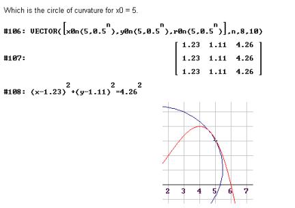
How to make tests for students
that are using a CAS tool (TI-89)
Bengt Åhlander
Trollhaettan, Sweden
3. Which polynomial fits to given points?
4. Approximation of square roots
6. Create and solve differential equations
7. Investigate the cubic functions
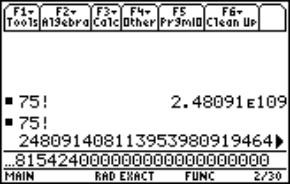
8. Why does 75! have 18 zeros in the end??
A little background to my teaching in math and physics for pupils 17 to 19 years old with the TI-89:
 All my students use the CAS tool TI-89
Every test my students have is divided into two
parts:
One part without any calculator and one part
with TI-89
The students must learn the basics with paper
and pencil
|
|
The new way to teach math with
CAS, Computer Algebra System, ¯¯¯ We have to face a new approach to make young students understand math better. ¯¯¯ One way is perhaps to give them
the answer of example from real life and let them make the right questions or
the right polynomials. ¯¯¯ |
|
Polynomial 1
|
The answer is: The quadratic function has 1 and 6 as zeros and the maximum value is 4. The question will be: What zeros and maximum value has
|
|
|
Fig. 1 |
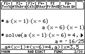
Polynomial 2
|
Randomly we make a quadratic function equal zero and solve it in one order. You get two solutions (zeros). Look at the window. Here from you ask your students if they can suggest one or two functions with these zeros. This is a way to make the students understand that every quadratic function can be at the form A(x-x1)(x-x2) |
|
|
Fig. 2 |
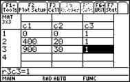
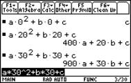
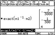
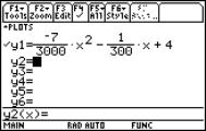
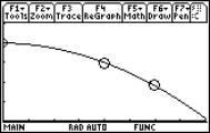
Which polynomial fits to given points?
You are standing with a snowball in a balcony 4 m
above the ground and want to hit your friend in the head 1,8 m above the ground
30 m away and you have to pass a 3m high wall 20m away.
Now you of course want to get the equation of
the parable the snowball made.
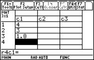
That means we want a polynomial that pass 3
points. (0,4); (20,3) and (30,1.8)
Then the students have to try what order on the
polynomial they need and then set up an equation system.
In this case we try with the polynomial Y
= A x^2 + B x + C
Look at the windows to follow the solution:
|
|
|
|
|||
|
|
|
|
|||
|
|
Fig. 3 |
|
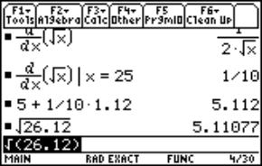
Approximation of square rootsCan you estimate a good value of Ö(26.12) when you know that Ö (25) = 5 without TI-89?????????????? |
|
|
|
Fig. 4 |
Bungy jump
A Coca-Cola tin filled with water tied up with an ordinary rubber band will be the model of a bungy jump. By releasing the tin over a CBR placed at the floor we can sample the movement with the graph calculator. The data we received can be analysed and a lot of calculations can take place.
|
|
|
|
|
|
|
|
|
Fig. 5 |
|
|
|
The students can use this graph as a homework to find the values of A, B, C and D: y = A sin(Bx + C) + D |
|
|
|
Fig. 6 |
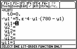
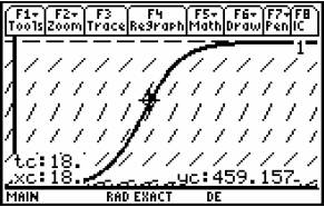
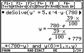
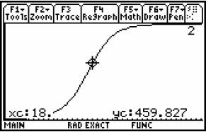
Create and solve differential equations
In a village with 780 people a rumour is
spreading with a velocity proportional to the number of people who do not know
it and the people that know. The speed is 0,05%.
Make a differential equation over the problem
and then solve it exactly and numerical with a slope field.
How many people know the rumour after 18 days?
This solution is a new way to such a problem,
both in a numerical and exact way.
|
|
|
|
Fig. 7 |
|
|
|
|
|
Fig. 8 |
|
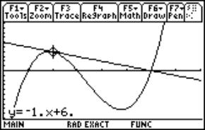
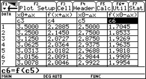
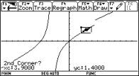
Investigate the cubic functions
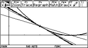
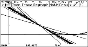
If you draw
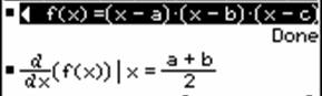
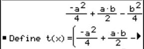
f(x) = (x-1)(x-3)(x-6) = x^3-10x^2+27x-18
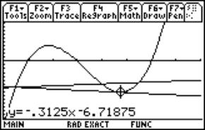
you discover the three zeros. If you take the mean value of two of the zeros and draw a tangent at this value you will hit the third zero with the tangent.
After
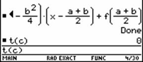
this investigation, I ask my students to show that this is true for all cubic
functions with three real zeros.
Here
is the CAS tool TI-89 really a good help.
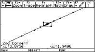
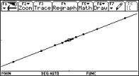
Perhaps
this is correct for every line, which has three intersections of the cubic
function?
|
|
|
|
|
Fig. 9a |
|
|
|
|
||
|
Fig. 9b |
Fig. 10 |
|
Why does 75! have 18 zeros in the end??
|
“Some mathematics becomes more important because technology requires it.— Some mathematics becomes less important because technology replaces it.— Some mathematics becomes possible because technology allows it.” Bert Waits. |
|
|
|
Fig. 11 |
Issues on integrating CAS in teaching mathematics:
A functional and programming approach
Halil Ardahan and Yaşar Ersoy
Konya, Ankara, Turkey
3. Digit spare function: formulation and applications
In recent years we have attempted to study main issues and various research questions about integrating and implementing cognitive tools such as computer algebra systems (CAS) environments, in particular TI-92 calculator in both teaching and learning mathematics in Turkey. In this presentation, after over viewing the main issues and obstacles on the subject matter very briefly, we construct a new function, named digit spare function (dsf), a functional approach to two digit prime numbers and a programming approach to find the greatest common divisor (gcd) of integers. Finally, we present a few instructional materials, which were designed and developed in the viewpoint of new learning theories and models, namely constructive and discovery learning.
1 Introduction
How do we solve problems, create new mathematical knowledge and teach it to students effectively? Is there an appropriate method and tool which helps people to solve real-life problems or give reasonable answers to such a particular questions? In this respect, G. Polya devised a problem-solving approach that guides students through the thinking process necessary for effective problem solving (Polya 1971). Although there are some strategies and ways to handle this sort of question there is no definite answer how to create new knowledge and solve real-life problems. Because problem solving involves more than exercises that use and practice algorithms. It consists of applying prior knowledge to find a possible solution for which there is no obvious path. But there are some cognitive tools which help us understand and create mathematics knowledge, and the ways we teach and learn mathematics. Among others, computer algebra systems (CAS) are tools, which automate the execution of algebraic computations, and enrich the teaching/learning environment. In the present paper, after giving a short summary of the issues on integrating CAS in teaching mathematics in Turkey, we study on creating a new function, namely digit spare function (dsf) to find greatest common divisor (gcd), a functional approach to two digit prime numbers and display a programming approach to find the greatest common divisor of integers. Finally, we will also present a few instructional materials, which were designed and developed in the viewpoint of new learning theories and models, namely constructive and discovery learning.
2 Background
Issues on using CAS environment in mathematics education
If someone follows the steps described in (Polya 1971) and use CAS appropriately he/she may create new mathematical knowledge, discover a set rules or get nothing new. For this purpose, advanced calculators and computers are valuable cognitive tools, i.e. for both creating new knowledge, teaching and learning mathematics, i.e. they enable us trivialisation, visualisation, experimentation and concentration in mathematics education (Kutzler 2000). This means that we can tackle more complex and more realistic problems and use “guess and chalk” strategy more effectively. This feature and potential should be taken into account to improve the present situation of mathematics education in Turkey as in other countries.
In the CAS teaching and learning environment, finding new functions, recognising and testing structures, visualisation and problem solving properly are indispensable skills and abilities (Herget e.a. 2000). In this case, a commonly held misconception is that if students are allowed to use computer and calculator technology, they will not able to perform calculations or understand mathematical reasoning without the aid of technology. Various research clearly dispels this myth. Therefore it is worthwhile to stress that one of the major impacts of such a technology on the mathematics curriculum is that it is now possible to introduce new topics simply because technology frees us from computations.
Finding prime numbers
The conventional, simple and most efficient way of finding small primes less than 10.000.000.000 is the way of using the Sieve of Eratosthenes. Make a list of all integers less or equal to n and strike out the multiples of all primes less or equal to the square root of n, then the numbers that are left are prime. Another way to find individual small primes trial division or wheel factorisation. To test n for primality just divide by all of the primes less than the square root of n
Also, many test are used to find primes like Pepin's Test, Lucas-Lehmar Test , etc.
The Euclidean algorithm to compute the greatest common divisor for two integers a and b (not zero) is based on the following fact. If r is the remainder when a is divided by b, then gcd(a,b) = gcd(b,r). This ancient algorithm was stated by Euclid in his Elements over 2000 years ago, and is still one of the most efficient ways to find the greatest common divisor of two integers. On modern computers the binary gcd algorithm is usually faster even though it takes more (but simpler) steps. One of the uses of the Euclidean algorithm is to solve the diophantene equation ax + by = c. This is solvable (for x and y) whenever gcd (a,b) divides c.
(http://www.utm.edu/research/primes/glossary/EuclideanAlgorithm.html).
3 Digit spare function: formulation and applications
The new way we propose to find the small prime numbers is the functional approach. Here the main question is "Can we write a function that selects the primes less than 100". Another question concerned with this is "How can we teach this subject to students by using calculators?" In the following section, there are some activities which were designed to answer these questions.
Digit spare function (dsf)
Problem: Can we construct a function that separates the digits of an integer with length n, nÎN?
Paper and Pencil Formulation: Let us begin a simple question to explain why we need a new function. For the illustrative purpose let us choose any whole number like 21. If we divide this integer by ten and calculate the remainder, we find out unit digit, 1. This process is valid for every whole number. Let us choose another integer like 321. If we divide this number by ten and calculate the quotient we find 32 and applying the above procedure we find the tens digit 2. Again, if we divide 321 by a hundred and take the integer part we find the hundreds digit 3. Now, let us choose the integer 4321. By using "mod" command with modulo 10 we find the units digit as follows: 1 = mod(4321,10). By using the "int" command we find the quotient as follows:
|
|
432 = int (4321/10) |
(1) |
By applying the "mod" command again on the quotient 432 we get
|
|
2 = mod (432,10) |
(2) |
as the tens digit of the integer 4321. If we combine the equations (1) and (2) we can write
|
|
2 = mod (int(4321/10), 10) |
(3) |
|
|
3 = mod (int(4321/100), 10) |
|
|
|
4 = mod (int(4321/1000), 10) |
Now, it is time to generalise the procedure. Let w be a whole number (w = 4321). Let n be the length of the integer w and let d(n) be the digits of the integer w. We can write the Algebraic model of the procedure and the equation (3) as follows:
|
|
d(n) = mod ( int (w/10LEN(w) ), 10), n = LEN(w) or |
(4) |
|
|
d(n) = mod ( int w/10n ), 10), n = 0,1,2, ... , LEN(w) |
where d(0)= units digit, d(1)= tens digit, d(2)=hundreds digit and so on.
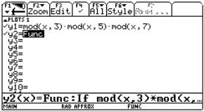
Use of Calculator: After we work out the problem, we are ready to construct the TI-92 model of the procedure. To do this we perform the following steps.
First,
we set the table parameters to: tblStart
=0, Dtbl=1 and press ENTER
.
Second,
we press on the Diamond [Y=] or APPS
2 to display Y= Editor and type the expression (4)
with default variable x and press ENTER . We get the screen shown in Fig 1, and by
pressing Diamond + TABLE buttons we can see the table
values of dsf.
|
|
|
|
Fig. 1 |
|

Again,
by pressing Diamond GRAPH
buttons we see the graph of dsf and its special properties displayed in
Fig 2.
|
|
|
|
Fig. 2 |
|
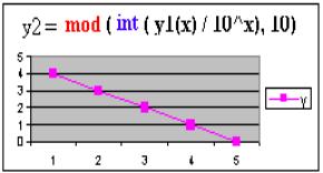
Notice. If the digits of an integer make arithmetic's sequence then the dsf is linear.
Applications of digit spare functions
Question 1: If the sum of digits of the two, three or more digit integer is divisible by three then the cubic sum of the digits is also divisible by three. Can you construct a model justifying the problem and generalise the result?
Solution. A functional approach by using TI-92 calculator.
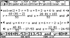
In the first step, let us construct the function, which generates the two digit integers divisible by three. This function is easily written as f(n) = 12 + 3 n , 0 £ n <30 and there are thirty integers in this set and the sum of digits of these integers is multiple of three. After, setting the table parameters to: tblStart =0, Dtbl=1, we can construct the TI-92 model of the problem and by pressing Diamond + TABLE buttons we see the values of the dsf as shown in Fig 3.
|
|
|
|
Fig. 3 a |
Fig. 3b |
What do you realise from the column y5 on the data table? May this result be valid for prime numbers? You can use this model to solve the problem for three digit numbers and others. Do you dare to establish the algebraic model for this problem?
|
Hint. |
If a + b = 3 n, nÎN then a3 + b3 = (a + b) 3 - 3 (a2 b + b2 a). If a + b + c = 3 n, nÎN then a3 + b3 + c3 = (a + b + c) 3 - 3(a2 b + b2 a + (a + b)2c + (a + b)c2) |
|
Now, we can generalise the results as follows. Let the length of an integer be n, nÎN. If the sum of the digits of an integer is divisible by tree then the sum of cubic power of the digits also divisible by tree.
Question 2: Can we construct a function, which generates the three digit integers having the sum of its digits seven? Can seven divide the sum of the seventh power of the digits?
Algebraic Model: Let us construct the algebraic model of the problem. When we examine the values of the function f(n) = 7 n, nÎN we see that, 106 is the least value and the sum of digits is seven. Similarly, the firs available number beginning with two hundred is 205; with three hundred is 307; with four hundred is 403; with five hundred is 502; with six hundred is 601 and the last number of these sequence is 700. The consecutive differences between the terms are constant and ninety-nine. The function which generates the sequence is f(n) = 106+99 n , n = 0,1,2, .., 6. In addition, the differences between the terms of the subsequence beginning with 106 are 9. That is to say, the function which generates this subsequence is f(n) = 106 + 9n, n = 0,1,2, .., 6. We can write the similar functions generating the other subsequences as follows; f(n) = 205 + 9n , n = 0,1,2, ..,5; f(n) = 304 + 9n , n = 0,1,2, .., 4; f(n) = 403+ 9n, n = 0,1, ... ,3; f(n) = 502+ 9n , n = 0,1,2; f(n) = 601 + 9n , n = 0,1; f(n) = 700 + 9n , n = 0.
Use of Calculator: Now, let us use TI-92 calculator to construct the model of the problem.
On
the Y= Editor we write the above
function with given conditions as follows;
|
|
|
|
|
|
Fig. 4a |
|
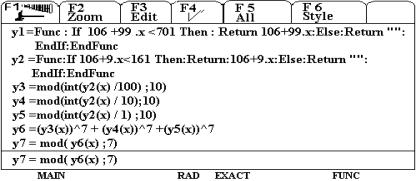
By pressing Diamond + TABLE buttons
we see data on the table.
|
|
|
|
|
|
Fig. 4b |
|
What do you realise from the column Y5 on the data table?
Result: The sum of seventh powers of the digits of a three digit numbers having the sum of seven divisible by seven.
Question 3: Do we write a function, which selects the two digit prime numbers?
Forming the function: A functional approach to two digits prime numbers.
The even numbers are not prime numbers except 2. Since the multiplication of two or more then two odd numbers is odd number, the prime factors of these numbers may only be three, five or seven. If the reminder of two digit odd numbers are multiplied and the multiplication is not zero then this odd number can not be divided by three, five or seven and it is prime number. So, if n is any two digits odd number then
|
|
p(n) = mod( n, 3) . mod( n, 5). mod( n, 7) |
(5) |
is a desired function.
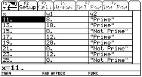
Using Calculator: Let us practice this function on TI-92 calculator.
In
the first step, we set the table parameters to: TblStart =11, Dtbl=2,
and press ENTER .
Second,
by pressing Diamond [Y=] buttons we see the function editor
and write the function following
functions and by pressing Diamond TABLE
buttons we see the results.
|
|
|
|
Fig. 5a |
Fig. 5b |
By
pressing Diamond GRAPH buttons
we see the graph of the function.
|
|
|
|
|
|
Fig. 6 |
|
By
setting the table parameters to:
ASK we can get special values and
the graph of dsf.
|
|
|
|
Fig. 7a |
Fig. 7b |
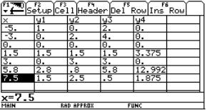
Is dsf defined on rational numbers? How can we explain the behaviour of the function for the rational numbers?
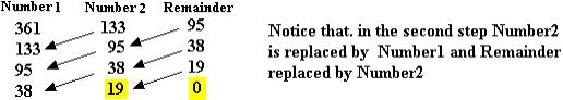
Question 4: Can you construct an algorithm or program to find the greatest common factor (gcf) of given two numbers using TI-92 Calculator? Then, find the gcf of 361 and 114 using TI-92 calculator.
Solution
Using
the Euclidian algorithm we can write the equation 361= 133´2 +
95.
The
gcf of 133 and
95 is also the gcf of 361 and 133.
So,
by using Euclidian algorithm once more we write 133 = 95´1 + 38 and 95 = 38´2+ 19.
If
we continue this process until the
remainder becoming zero, we find the gcf of
given two integers.
Now,
we construct a data table to find the relation among the data.
|
|
|
|
|
|
Fig. 8 |
|
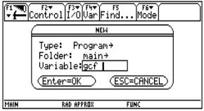
Considering
the above algorithm we can write a program for the procedure with TI-92 to find
the gcf of 361 and 114 as 19.
After
pressing APPS + 7 + 3 buttons we can write the following
program.
|
|
|
|
|
|
Fig. 9 |
|
: gcf ( )
: prgm " Calculation of GCF"
: Input " Input first integer (n1)", n1
: Input " Input second integer n2 (n2 > n1)", n2
: For i, 1, n2, 1
: Label REMAINDER
: mod (n1,n2) STO ® r
: If r > 0 Then
: n2 STO ® n1
: r STO ® n2
: goto REMAINDER
: Else
: End IF
: EndFor
: Disp " gcf = " , n2
: End Prgm
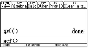
To
get the outputs of the program press Diamond HOME
and write
"gcf ( )" on the formula bar and press ENTER . (see Fig. 10a). When you
input the numbers 247 and 114 you will see the desired results (in Fig. 10b).
|
|
|
|
Fig. 10a |
Fig. 10b |

If the remainders are not zero in the program what happen? Can you explain it?
We tried to solve three types of problems with different approaches with CAS. If the functional and linear algorithm is fail to solve a problem then we should use programming approach of TI-92 / CAS.
4 Concluding remarks
In the present study, we focus on the design of particular instructional materials on number theory, and guide the learners how to use the cognitive tools and create new mathematical knowledge. To answer such a question, we help student teachers and practising teachers use CAS environment, in particular TI-92 calculator, and work out the details for constructing the model of solving certain problems. Thus, the use of the calculator is integrated to teaching and learning of mathematics throughout the examples. In the seminar and workshop organised in Turkey, we have got some experiences and the impression that if a learner performs the requested tasks carefully he (she) will explore concepts him/herself and may discover a new relationship, rule or theorem in CAS environment. To do this, both the instructors and learners, however, need some competencies, effective cognitive tools, and samples of instructional materials, etc.
Moreover, we share the view that there is no longer a question as to whether computers and calculators should be used in the learning and teaching of mathematics, but this technology should be available for all students (Standards 1989). Because CAS environments, either calculators or computers, let students solve challenging problems that would otherwise take too much time with paper and pencil. Thus, students are better able to manage the over-all problem solving process when they are expanding less energy on its computational aspects. The “guess and check” strategy also becomes a more realistic approach when technology removes the drudgery of recalculating results with different inputs.
References
Polya, G. (1971) How to solve it. Princeton University. Princeton, New Jersey.
Kuzler,B. The algebraic calculator as a pedagogical tool for teaching mathematics. Laughbaum, E. (ed) (2000) Hand-Held Technology in Mathematics and Science Education: A Collection of Papers. Ohio State Uni. Pub., Columbus, 98-109.
Herget, W.,Heugl, H., Kuzler,B., Lehmann, E. (2000) Indispensible manuel skills in CAS environment. Kokol-Voljc, V. e.a. (eds) Proceedings of ACDCA-6, Hagenberg: bk teachware Lehrmittel, 13-26.
http://www.utm.edu/research/primes/glossary/EuclideanAlgorithm.html.
Standards (1989) Curriculum and Evaluation Standards for School Mathematics. National Council of Teachers of Mathematics (NCTM) Pub., Reston, Virginia.
Animiertes Grafiken-Zusammenspiel
von PC und TC in der Mathematik
Detlef Berntzen
Münster, Germany
1. Vorbemerkungen sowie Hardware- und Softwarevoraussetzungen
2. Arbeitsschritte zur Produktion eines animierten GIF-Bildes
4. Ein ausgearbeitetes Beispiel: Die aufblühende Potenzblume
Die Zentrale Koordination Lehrerausbildung der Westfälischen Wilhelms-Universität Münster führt seit 1996 das Lehrerfortbildungsprojekt „Teachers Teaching with Technology“ durch (vgl. Berntzen 2000). In diesem Projekt werden vorwiegend MathematiklehrerInnen mit dem Umgang moderner Technologien und deren mathematisch-sinnvollen Einsatz im Unterricht geschult. Eine zentrale Rolle in den Schulungen spielen dabei Taschenrechner, die den LehrerInnen und SchülerInnen mathematische Expertensysteme (Computeralgebrasysteme, dynamische Geometriesoftware, Spreadsheets) im handheld-Format zur Verfügung stellen. Eine technologische Spitzenstellung nimmt dabei der Taschencomputer TI‑92 der Firma Texas Instruments ein.
1 Vorbemerkungen sowie Hardware- und Softwarevoraussetzungen
In diesem Artikel wird vorgestellt, wie man mit Hilfe des Taschencomputers TI-92 im Zusammenspiel mit einem Windows-PC animierte Grafiken erstellen kann, die wiederum dazu dienen (können), erarbeitete mathematische Zusammenhänge zu illustrieren. Im ersten Schritt werden an einem einfachen Beispiel die programmtechnische Basis und die notwendige Hardwarekonfiguration vorgestellt. Diese benötigt man, um kleine mathematische GIF-Filme – animierte GIF-Images – zu produzieren. Danach werden in einem zweiten Schritt mögliche Anwendungen dieser Technik für den Mathematikunterricht in der Schule sowie in der Aus- und Fortbildung von MathematiklehrerInnen erörtert.
Das unten angeführte Beispiel wurde mit einem Taschencomputer TI-92 plus und einem D21-PC (IBM Aptive mit Windows 98) sowie einem Graphlink-Kabel als Verbindung zwischen der I/0-Schnittstelle des TI-92 plus und dem freien COM-Port (serielle Schnittstelle) durchgeführt. Man kann vergleichbar mit jedem Windows-PC ab Win 3.1 arbeiten. Statt des TI-92 plus kann alternativ ab TI-83 die gesamte Palette von Graphikrechnern von Texas Instruments benutzt werden. Für das Beispiel wurde auf dem PC folgende Software eingesetzt:
TI
Link-Software (frei verfügbar, i.d.R. mit dem Graphlink-Kabel mitgeliefert);
IrfanView
(Sharewareprogramm zur Konvertierung von Graphikdateien);
Gifcon
32 (GIF-Konstruktionssoftware als Shareware im Internet downloadbar).
2 Arbeitsschritte zur Produktion eines animierten GIF-Bildes
Zunächst werden Screenshots vom TI-92 plus mit Hilfe der TI Link-Software geschossen und im TIF-Format auf dem PC – am besten in einem eigens eingerichteten Ordner – angelegt. Diese TIF-Dateien werden durch das Programm IrfanView ins Bitmap-Format konvertiert. Die bmp-Files werden anschließend mit dem Gifcon 32-Programm zu einem Film zusammengestellt. Diese drei Arbeitsschritte werden im Folgenden näher erläutert.
Produktion der Screenshots
Die TI-Link-Software ermöglicht, Screenshots vom TI-92 plus im TIF-Format aufzuzeichnen. Um einen vollständigen Eindruck der Vorgehensweise bei der Lösung eines mathematischen Problems mit diesem Taschencomputer erzeugen zu können, muss nach jeder Tastatureingabe ein Screenshot aufgezeichnet werden.
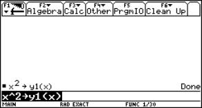
|
D.h., um die Funktionsdefinition x^2 ® y1 (x) im Home-Screen des TI-92 plus aufzeichnen zu wollen, müssen – inkl. leerem Bildschirm – 10 Einzelbilder gespeichert werden. |
|
|
|
Fig. 1 |
|
Das Eingeben und Lösen von linearen Gleichungen der Form 5x + 6 = 3x – 2 erfordert ca. 20 Bildschirmschnappschüsse. |
|
|
|
Fig. 2 |
Ein kleines Projekt – etwa das Erzeugen von 100 Zufallszahlen im Dateneditor in einer Spalte und das Erzeugen von weiteren Berechnungsspalten im selben Dateneditor mit anschließender grafischer Datenauswertung – erzeugt einen Bestand von etwa 100 einzelnen Screenshots. Leider gibt es keine Software, die automatisch nach jedem Knopfdruck am Taschencomputer einen Screenshot aufzeichnet und ihn mit durchlaufender Nummerierung in einen vorgewählten Ordner unter Windows ablegt. Ein solches unterstützendes Programm ist bei Texas Instruments als Desiderat angemeldet worden.
Das Konvertieren des Screenshots
Als Konvertierungsprogramm wird das Shareware-Programm „IrfanView“ aufgerufen. Das Programm ermöglicht die Batchkonvertierung der Screenshots. Auf Grund der verwendeten Software zur Erzeugung animierter GIFs, die das TIF-Format nicht erkennt, ist eine Konvertierung notwendig.
Von den Einzelbildern zum animierten GIF
Dieser letzte Produktionsschritt ist relativ schnell durchzuführen. Das Programm „GIF Construction Set 32“ stellt unter dem Menü-Punkt „Animation Wizard“ ein Tool zur Erzeugung animierter GIFs zur Verfügung, nach dessen Aufruf man einige Voreinstellungen treffen muss:
Der
GIF-File ist für das WWW ausgelegt;
der
GIF-File kann beliebig oft wiederholt oder nach einmaligem Durchlauf gestoppt
werden;
die
Dateien, die verwendet werden, sind photorealistisch.
Anschließend wird man aufgefordert, die Verzögerung zwischen den Einzelbildern vorzuwählen. Hier sollte man 1/10 Sekunde – wie vorgeschlagen – beibehalten. Man kann dies nachträglich an den Stellen ändern, an denen längeres betrachtendes Verweilen erwünscht ist – zum Beispiel am Ende von Eingaben oder zum Betrachten von Grafiken.
Jetzt kann man die Bilddateien auswählen, die in der Animation auftreten sollen. Im Dateifenster wird dieses durch Doppelklicken der Dateien erreicht – ohne das Fenster jeweils verlassen zu müssen. Das GIF-Construction Set zeichnet die Auswahl auf. Damit ist die Arbeit getan und das GIF-Tool erzeugt die Animation selbständig. In der Vorschau – View-Button – kann man sein animiertes GIF nun betrachten. Will man die Einblendezeit eines Bildes ändern, wählt man mit der Maus die CONTROL-Zeile, die über dem Bild steht, per Doppelklick aus und wählt den „Delay“ neu.
3 Anwendungsgebiete
|
Die animierten GIFs aus TI-92 plus-Bildern eignen sich für die Präsentation von Beispielrechnungen auf dem Taschencomputer im Internet. Komprimierte Files – etwa das oben erwähnte Beispiel zum Gesetz der großen Zahlen – sind Filme von 2 Minuten Länge, die aber nur 64 Kbyte Dateigröße besitzen. Sie haben die angenehme Eigenschaft, dass sie mit dem Abspielen der Gesamtsequenz starten, bevor der File komplett über das Internet heruntergeladen ist. |
|
|
Fig. 3 |
Diese GIF-Filme sind nicht selbsterklärend, sie müssen mit entsprechenden Kommentaren versehen werden. Sie helfen, im Selbststudium den technischen Umgang mit dem TI-92 plus zu erlernen. Die Materialien, die einem solchen Konzept entsprechen, können natürlich auf CD-Rom abgelegt werden.
Die Produktion von Medien – Webseiten mit animierten GIFs entsprechen dem Konzept von Multimedia im Sinne der Verknüpfung von Text und bewegtem Bild (vgl. Breger und Grob 1999 und Strittmatter und Niegemann 2000) – kann Ziel in vielerlei Lehr‑/Lernkontexten sein. Im Sommersemester 2001 hat der Autor ein fachdidaktisches Seminar für Lehramtsstudierende der Mathematik (Sek II und Sek I) angeboten, in dem diese Form der Medienproduktion in den Mittelpunkt gestellt wird. Eine derartige Veranstaltung kann damit in den an der Universität Münster geplanten Zusatzstudiengang „Medien und Informationstechnologien in Erziehung, Unterricht und Bildung“ eingebunden werden. Für diesen Zusatzstudiengang ist ein Leistungsnachweis durch eine Medienproduktion – ggfs. im Rahmen einer Gruppenarbeit – obligatorisch.
Darüber hinaus kann die Produktion von animierten GIFs auch im Mathematikunterricht von SchülerInnen durchgeführt werden. Ein entsprechendes Austauschprojekt zwischen den Studierenden des oben erwähnten Seminars und einer Schule in Münster wird angestrebt. Des weiteren sollen die im obigen Rahmen erstellten Medien im Lehrerfortbildungsprojekt „Teachers Teaching with Technology Deutschland“ zum Einsatz kommen.
4 Ein ausgearbeitetes Beispiel: Die aufblühende Potenzblume
Die mathematischen Grundlagen
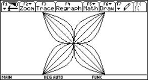
Die aufblühende Potenzblume, siehe auch
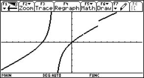
http://www.zkl.uni-muenster.de/Berntzen/SS2001/Potenzblume/, entsteht durch zentrische Streckung aus einer Grundfigur, der Potenzblume. Diese Grundfigur entsteht selber aus abschnittsweise definierten Potenzfunktionen mit den Exponenten 2,4,0.5 und 0.25 sowie aus abschnittsweise definierten linearen Funktionen x und -x. Beider Definition der Funktionen im Y=-Editor des TI-92 plus kann man die Symmetrieeigenschaften der Funktionen - und diese spiegeln sich in der Potenzblume wider – benutzen.
Die graphische UmsetzungIm Y=-Editor des TI-92 plus lässt sich die Grundfigur wie folgt definieren:
|
Fig. 4 |
||||||||||
jeweils eingeschränkt auf das Intervall [-1,1]; die Grundfigur sieht demnach wie abgebildet aus. Für die zentrischen Streckungen muss man beachten, dass eine Funktion y(x) mit dem Definitionsbereich [-1,1] bei Streckung um den Ursprung mit dem Faktor a in eine Funktion ya(x) = a y(x/a) mit Definitionsbereich [-a,a] übergeht. |
Die technischen Details
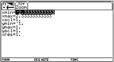
Um die graphischen Fähigkeiten des TI-92 plus vollständig auszunutzen, sind für die Grundfigur folgende Einstellungen im Window-Menü des Taschencomputers optimal: Sie sorgen für eine verzerrungsfreie Darstellung der Potenzblume in voller Ausnutzung der Fenstergröße. Durch die Wahl xres=1 wird dafür gesorgt, dass die Auflösung des Bildschirms maximal ausgenutzt wird. Über F1/Format werden im Graphik-Fenster zudem alle Graphikelemente (Grids, Achsen, Beschriftungen) ausgeschaltet.
|
Durch den im Homebereich festzulegenden Streckungsfaktor a lassen sich sukzessive Abbilder der Grundfigur mit a = 0.1, 0.2, ..., 1.0 im Graphikfenster darstellen. Der Aufbau jedes dieser Bilder dauert einige Minuten. Schnellerer Bildaufbau lässt sich nur zu Lasten der Auflösung erreichen (z.B. durch Heraufsetzen von xres im Window-Fenster). |
|
|
Fig. 5 |
Überlegungen zur methodisch-didaktischen Umsetzung im Unterricht
Die Grundfigur der Potenzblume und ihren methodisch-didaktischen Hintergrund kann man in Barzel (1999) nachlesen. Die dort aufgeführten Möglichkeiten werden durch folgende Elemente ergänzt:
mathematisch-inhaltlich:
zentrische Streckung
Arbeitsform:
Projektarbeit zur Erstellung des animierten Gifs.
Der zweite Punkt lässt Variationen zum oben gezeigten Film zu: Man reduziere die Grundfigur auf die Exponenten 4 und 1/4 und führe für diese Figur die zentrischen Streckung durch. Anschließend entfalte man die neue Grundfigur zur vollen Potenzblume durch Variation der Exponenten! Man wähle andere Figuren aus Barzel (1999) und bewege diese auf dem Bildschirm durch Verschiebung oder Drehung! Man wähle ein einfaches Logo und simuliere die Drehung - als Projektion der Drehfigur auf die Graphikfläche des Taschencomputers! Die Idee stammt von Laakmann.
Links
Die Homepage der Firma Texas Instruments findet man unter der URL
Die Homepage zu Gif Constructionset 32 findet man unter
References
Barzel, B. e a.(1999) Neue Technologien- Neue Wege im Mathematikunterricht. Linz
Berntzen, D. (2000) Teachers Teaching with Technology Deutschland. Genese und Organisation eines Lehrerfortbildungsprojekts. Münster.
Breger, W. Grob and H.L. (1999) Präsentieren mit und ohne Multimedia. Mit Beiträgen von Rüdiger Ganslandt, Alexander Güttler und Klaus Linneweh. Münster.
Grob, H.L. and Bieletzke, S. (1997) Aufbruch in die Informationsgesellschaft. Münster.
Laakmann, H. Private Kommunikation nach diversen Unterrichtsbesuchen im Annette-von-Droste-Hülshoff-Gymnasium Münster.
Strittmatter, P. and Niegemann, H. (2000) Lehren und Lernen mit Medien. Eine Einführung. Darmstadt.
From pole to pole – A numerical journey
to an analytical destination
Josef Böhm
Würmla, Austria
2. A numerical approach to the instantaneous rate of change
3. Curvature on the spread sheet
The TI-89/92´s Data/Matrix-editor is an excellent tool to support concepts of accumulation points, limits, continuity, average and instantaneous rates of change. Some steps can be done using a spreadsheet, too. But very soon we miss the comfortable use of functions and much more important the computer algebra. In this paper we focus on the use of handheld technology, because we experienced the advantage of the overall and anytime availability of these small machines. The author tried the same approach with a calculus class in the PC-lab using DeriveÔ.
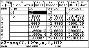
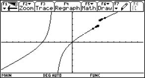
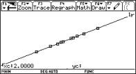
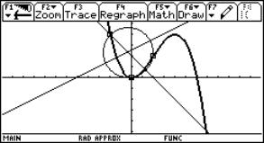
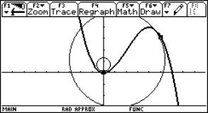
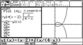
1 An exotic function
|
Let me start discussing continuity using an "exotic" function:
Which values for x are excluded from the domain? To keep the exploration as general as possible I recommend to store the function as f(x) in the Home Screen. Then open a new Data Sheet via the Data/Matrix Editor, say analysis. |
|
|
Fig. 1: Graph of the exotic function |
Continuity behaviour at x0 = 3
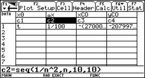
|
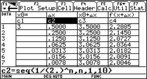
In cell c1 we enter the value of x0. In column c2 we define a 0-sequence to obtain in c3 a sequence of x-values with right side limit 3. Subsequently in c4 we can see the sequence of function values, which should tend to f(x0). (Experiment by changing the sequence in c2). For c3 enter: c1[1]+c2 For c4 enter: f(c3) In columns c5 and c6 we generate the left sided approach. How should we change c2 to accelerate the convergence behaviour? |
|
|
Fig. 2a |
|
|
|
|
|
Fig. 2b |
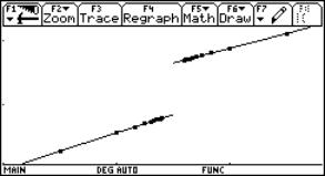
Using the plot-facilities we can visualize the convergence process:
|
|
|
|
|
Fig. 3: Zooming to investigate the continuity behaviour at x0=3 |
||
Continuity behaviour at x0 = -3
|
|
|
|
Fig. 4a |
Fig. 4b |
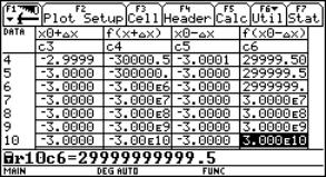
The results in columns c4 and c6 are very informative!!
Continuity behaviour at x0 = 4.5
|
|
|
|
Fig. 5a |
Fig. 5b |
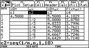
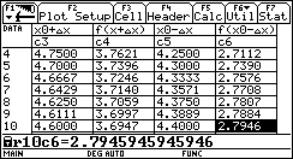
Discuss the outcomes in columns c4 and c6. Change the sequence in c2. Discuss possible consequences. Produce a graphic representation.
|
|
|
|
Fig. 5c |
Fig. 5d |
The last interesting position is x0 = 2
|
|
|
|
|
Fig. 6: Zooming to investigate the continuity behaviour at x0=2 |
||
Discuss all the information given on the screen
Continuity can be discussed more or less successfully using a spreadsheet. Unfortunately the graph could be misleading. The tables are also showing strange results. See one example:
Behaviour for x0 = 4.5:
|
n |
Dx=0.5^n |
x0 + Dx |
f(x0 + Dx) |
x0 - Dx |
f(x0 - Dx) |
|
16 |
1,5259E-05 |
4,50001526 |
3,65000682 |
4,49998474 |
2,84999156 |
|
17 |
7,6294E-06 |
4,50000763 |
3,65000341 |
4,49999237 |
2,84999578 |
|
18 |
3,8147E-06 |
4,50000381 |
3,6500017 |
4,49999619 |
2,84999789 |
|
19 |
1,9073E-06 |
4,50000191 |
3,65000085 |
4,49999809 |
2,84999894 |
|
20 |
9,5367E-07 |
4,50000095 |
3,65000043 |
4,49999905 |
2,84999947 |
Using another sequence for the Dx, we find a "convergence" towards the average of left- and rightsided last values!!
|
1E-14 |
4,5 |
3,65 |
4,5 |
2,85 |
|
1E-15 |
4,5 |
3,65 |
4,5 |
2,85 |
|
1E-16 |
4,5 |
3,25 |
4,5 |
3,25 |
|
1E-17 |
4,5 |
3,25 |
4,5 |
3,25 |
Working with a CAS DERIVE doesn´t show significant differences to the TI´s results. One cannot work with the spreadsheet like DATA-Editor, but use the VECTOR-and TABLE command to produce tables. This will be shown later in this text.
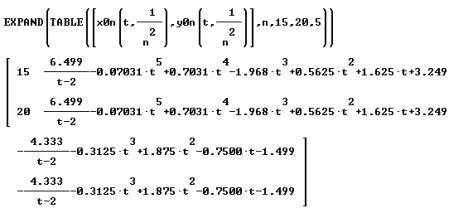
2 A numerical approach to the instantaneous rate of change
Now it is easy to extend this table for further use in calculus teaching. We only have to add some columns for the absolute changes and then for the rates of change leading to the average rate of change and to its limit.
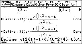
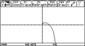
Let’s have another "artificial" function. Do you know the "MM Curve"?
![]()
|
|
|
|
Fig. 7a: x0 = 2 |
Fig. 7b: x0 = 0 |

Can you see a difference in the behaviour of the rates of change comparing the tables?
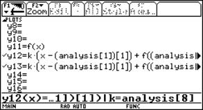
We use the left- and right-sided difference quotients (rates of change) to plot the families of secants. First for x0 = 2 (use the values from the DATA sheet to define a family of secants):
|
|
|
|
Fig. 8a |
Fig. 8b: Left sided approach |
|
|
|
|
Fig. 8c: Right sided approach |
Fig. 8d: Both families |
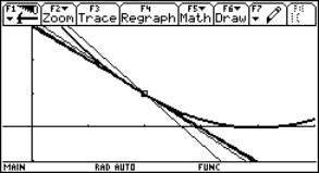
Use various sequences for approaching x0 = 0. Is the function continuous for x0 = 0?
Plot the two families of secants and comment their end behaviour. Can you predict the tangent in (0 / 4)?
|
|
|
|
Fig. 9: Left and right sided secants and tangents in (0,4) |
|
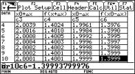
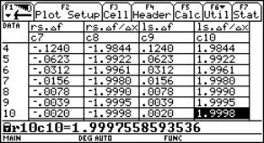
Further exploring:
|
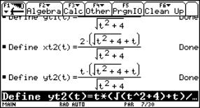
Try another function, e.g.
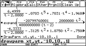
Perform the same investigation like above, but finally enter x0 = t for the location: Attach one more column to expand the results from c10 or c8. Copy and paste content of cell r10c11 into the Home screen and try to make conclusions for a general rule to find a formula for the instantaneous rate of change. On earlier TI-versions you cannot copy the content. Switch to the Home screen and enter analysis[11][10] to see the result. |
|
|
Fig. 10: To find a formula for the instantaneous rate of change |
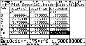
Describe also the "last" elements in columns c4 and c6 - repeating and deepening continuity. The last part – 7.5 * 10-11 is so small, that it has practically no influence on the result, so it can be neglected.
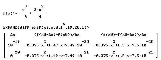
Using DERIVE the students also receive an impressive insight. It is a challenge to produce powerful functions for calculating the difference quotients, put them in tables and use the values for plotting the secants. See a part of the respective DERIVE session.
This table has a similar structure as a part of the TI-DATA-sheet. In the following we omit columns 2 and 3 and show only the Dx together with the sequences of both difference quotients.
|
|
|
|
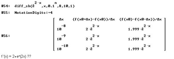
It is very nice to "derive" the derivatives of the most important functions using the capabilities of a CAS. See one example, how it works with sin x:
|
|
|
|

It is one of the fundamental ideas in numerical and applied mathematics to neglect small numbers to achieve a useful result. Another example to prepare the students for the chain rule:
|
|
|
|
To make it clear, I don´t want to substitute mathematical proofs by numerical investigations, but procedures like these might improve the students imagination about average and instantaneous rate of change and open their minds for the basics of analysis.
Using the TI, DERIVE or any other CAS it is no problem to proceed going one step further than usually in Secondary School.
3 Curvature on the spread sheet
|
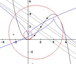
It is a challenge to find the circle of curvature in this way, i.e. without treating this question in the usual way determining the centre of the osculating circle as the limit position of the intersection point of two neighbouring normals of the curve. As I want to extend the Dx approach - without working with the 1st derivative I am not able to set up the equation of the normal line of a function graph. |
|
|
Fig. 11: Midpoint of osculating circle by intersection of two neighbouring normals |
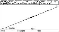
We will take the function from before and make further use of our created DATA sheet analysis. We want to find the osculating circle on locations x0 = 0, x0 = 1 and again generalized on x0 = t. Take three points on the graph
(x0-Dx, f(x0-Dx)), (x0, f(x0)) and (x0+Dx, f(x0+Dx))
and find the circumcircle. If Dx tends to 0 the circle will have three points in common with the graph - the osculating circle.
Where is the centre of this circle? What is its radius?
The centre is the limit of the intersection of the two perpendicular bisectors (see the TI-plo above). Again we extend the DATA sheet. But now we use the power of a CAS. Define a function pbi(x0,h,x) for the perpendicular bisector of the segment
[ (x0, f(x0)), (x0+h, f(x0+h)) ]
and calculate the first coordinate of the intersection point of pbi(x0,h,x) with pbi(x0,-h,x). Store the result as xco(x0,h) (h is equivalent to Dx).
|
|
|
|
Fig. 12: Table for x0 = 0 (c1[1] = 0) |
|
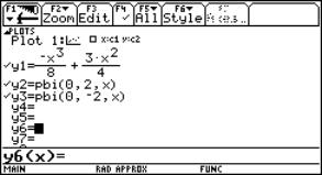
- x ^ 3 / 8 + 3 *
x ^ 2 / 4 → f ( x )
- h / ( f ( x0 + h) – f ( x0 ) ) * ( x - ( 2 * x0 + h ) / 2 ) +
zeros ( pbi ( x0, h, x ) – pbi ( x0, - h, x ) ,
x ) [ 1 ]
ans ( 1 ) → xco ( x0, h )
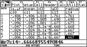
Now switch to the Data/Matrix Editor and attach two columns c12 and c13.
The header of columnc12 is c12 = xco(c1[1],c2) and the header of c13 is bi(c1[1],c2,c12).
In c14 you find the radius of the osculating circle (distance between point on curve and centre point). All values in c12, c13 and c14 seem to "meet" at (0, 2/3, 2/3).
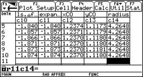
|
|
|
|
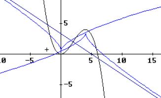
Fig. 13: Table for x0=5 (with c1[1] = 5) and the graph with the approximation of the circles |
|
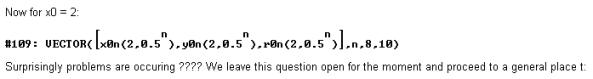
For completely generalized recalculation it is recommended to open a new DATA sheet to avoid memory problems. Then one needs only four columns and to display only the last row of the table. (Hint for the users: For switching here and back between Home screen and Data/Matrix Editor you should switch Auto Calculation Off).
|
|
|
|
Fig. 14: Generalized recalculation for the curvature |
|
|
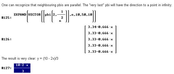
It should be a challenge for the students to investigate the behaviour of this curve for t = 2. Without having mentioned an "inflection point" ever before they have the chance to explore this very special point of a graph on their own. Find the asymptote of the "evolute" (= locus of the circle centres). |
|
|
|
Fig.15: The evolute – Locus of circle centres |
|
Here our roundtrip ends. We started investigating discontinuities finding a pole among them and we finish investigating a pole again. I think that we made an interesting journey into analysis. It is obvious that we have not really reached our destination point. Using the limits we obtain exact answers to confirm our numerical and graphical outcomes. |
|
|
Fig. 16 |
It is my experience that students like to follow this very "inner mathematical" reasoning. They feel their adventures in their heads and get a bit infected by the spirit of mathematics.
I want to give full credit to David Bowers who gave a marvellous workshop in San Francisco and in Liverpool as well showing so many possibilities how to use the TI´s Data/Matrix Editor in a very meaningful way. I also want to give credit to participants of the 1st T3 Winter Academy in Austria (1 - 6 January 2001), who gave the idea of "absolute adressing" a cell in the Data/Matrix Editor. (K.H. Keunecke, Detlev Kirmse, Manfred Grote). And once more to K.H. Keunecke, because his paper "Curvature" inspired me to extend my investigation of discontinuities to curvature.
I have nice memories of Jim Schultz´s (University of Ohio) visit in my school. He was witness when I first tried this teaching unit in two of my classes (without treating curvature!). At the evening we had interesting talks concerning the reactions of the students and the benefits of combining numerical and graphical approaches "preparing the ground" for exact definitions and proofs.
To give some impressions of the DERIVE version I add some sections from a DfW-file.
|
|
|
|
|
|
|
|
|
|
|
|
|
|
|
|
Fig. 17 |
Fig. 18 |
|
|
|
|
|
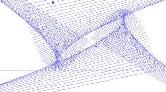
The reader is friendly invited to ask for the full paper containing further investigations (discontinuity of the curvature,…) at |
|
|
|
Fig. 19: The family of radii of the circles of osculation appears as a nice pattern of lines |
References
Böhm J. (2001) From Pole to Pole on the Data-Editor. Derive Newsletter 41.
Bowers, D. The Best of Two Worlds. Lecture on the ICTCM 12, San Francisco.
Keunecke, K.-H. (2001 ) Curvature as a Limit. Derive Newsletter 41.
Fermat’s Little Theorem
A thing of beauty is a joy for ever
John Cosgrave
Dublin, Ireland
“A thing of beauty is a joy forever.
Its loveliness increases; it will never
Pass into nothingness.”
John Keats (1795-1821), Endymion (1818)
This brief note is no more than an extended abstract for the Maple-presented talk I will give at the ICTMT 5 meeting in the University of Klagenfurt, Austria, in the week 5th-9th August 2001, the week before the 400th anniversary of Fermat’s birth.[1]
My Maple worksheet will contain a great deal more than I can cover in a 30-minute talk; it will be in active wms format–and so may be altered to suit the purposes of any interested reader–and also in html text format, and so it may be read by anyone who does not have Maple. I will place all versions in the Public and Other Lectures section of my web site
http://www.spd.dcu.ie/johnbcos
Fermat’s ‘little’ theorem is that if p is any prime, and a is any integer not divisible by p, then a p-1 leaves remainder 1 on division by p.[2]
In the language of congruences it is that
|
|
|
|
or that
|
|
|
|
It is one of the truly great theorems. Its congruence-free statement is extraordinarily simple, and could be explained to almost anyone, even to quite young children.
For the general public Fermat’s best-known theorem is, of course, his renowned ‘Last Theorem,’ which attracted wide media coverage at the end of the last century following the historic work of Andrew Wiles. However, while a proof of Fermat’s ‘Last Theorem’ required mathematics of extraordinary depth and difficulty, I don’t believe that anyone would argue that his Last Theorem is of any immediate value in terms of further consequences. In contrast, his little theorem has a huge number of important purely mathematical consequences, and practical applications. The purpose of the text of my talk is to draw together into a single document–perhaps for the first time – an identification of those disparate, important, and indeed fundamental applications. My document is intended to give pointers to further study for a reader who might not be well versed in Number Theory. [3]
For my Klagenfurt talk I have prepared a Maple worksheet in which I attempt to cover all that I believe is worth recording about it, and the gist of my talk may be gleaned from the sections into which I have divided it:
Section
1. The theorem itself, and how it originated.
Section
2. Decimal and other expansions of rational numbers.
Section
3. Quadratic and other congruences. Mersenne and Fermat numbers.
Section
4. Primality testing.
Section
5. RSA public-key cryptography.
Section
6. Factoring: Pollard’s (p - 1) factoring method.
Section
7. Open problems: primitive roots and Fermat numbers.
Section
8. Proofs of some important consequences of Fermat’s little theorem.
Section
9. Bibliography and web references.
References
Cosgrave, J. web site: http://www.spd.dcu.ie/johnbcos
Mahoney, M. S. (1994) The Mathematical Career of Pierre de Fermat. Princeton Univ. Press, 2nd ed.
Elimination of parameters and substitution with computer algebra
Guido Herweyers and Dirk Janssens
Oostende, Leuven
3. Cartesian equation of a plane
1 Introduction
Starting with the geometrical concept of parametric equations of lines and planes, we illustrate the method of elimination to obtain a Cartesian equation. This elimination can be done in a direct and simple way by using the procedures "solve" and "substitute" (the basic algebraic manipulations of formulas) of a computer algebra system (CAS).
Without a CAS this method is difficult to realize by hand (e.g. solution of a system of two equations for two of the four occurring "letters"). Therefore it was necessary to introduce in advance more elegant (but also more sophisticated) algebraic techniques like determinants. The result was that, for a lot of students, the meaning of the elimination process disappeared behind these algebraic manipulations. Later on in the educational process, we have the opportunity to show the equivalence and strength of the new algebraic techniques.
These ideas will be illustrated in a few (geometric) examples. The students should have as CAS a TI-92 or TI-89 at their disposal. With the commands "SOLVE" and " | " (substitute) one can obtain parametric equations from a Cartesian equation and vice versa.
2 A line in space
Find Cartesian equations of the line A with parametric equations
|
|
|
|

We obtain a point (x,y,z) of the line for each real value of the parameter t. For t = 0 we find the point (2,5,1) and for t = 2 the point (4,13,19) of the line. As t runs over R, the point (x, y, z) runs over the complete line A. Vice versa, a given point (x, y, z) will lie on the line if we find a value for t that satisfies the given equations. For example, the point p(13, 49, 100) will lie on A if the system
|
|
|
|

|
has a solution for t. We can verify this by solving the first equation for t (this yields t = 11) and substituting this value in the two last equations. These conditions are fulfilled, thus p lies on A. Finding Cartesian equations of a line means that we have to find the conditions for the coordinates (x, y, z) of a general point in order that the system would have a solution for t; we eliminate the parameter t. |
|
|
Fig. 1 |
We can use the same procedure as for that concrete point. First we enter the equations into the calculator (see Fig.1).
We solve the first equation for t. One can copy the equation with the ENTER key. Then we substitute t in the other equations. One can also copy the expression t = x – 2 with ENTER.
|
|
|
|
Fig. 2 |
Fig. 3 |
We see that the line A is described as the intersection of two planes:
|
|
|
|
We can use the same method to find a Cartesian equation for a plane with given parametric equations.
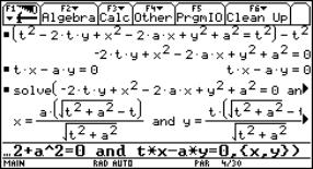
3 Cartesian equation of a plane
|
Find a Cartesian equation of the plane a with parametric equations Again we start with entering the three equations. We now use the two first equations to solve them for r and s. |
|
|
Fig. 4 |
 .
. 
One can enter a system into the SOLVE command by connecting the equations with "and". Put the variables we are solving for between braces. We now substitute these expressions in the third equation. Most can be done by copying the obtained expressions. Possibly we get rid of the denominators.
|
|
|
|
Fig. 5 |
Fig. 6 |
The plane a has the equation 45x + 25y – 24z –471 = 0.
4 Intersection of two planes
Find parametric equations for the intersecting line A of the planes
|
|
|
and |
|
|
The choice of letters for parameters is essentially free, but misleading in the given situation because we are describing the two planes with the same letters r and s . Equal parametric values yield different points of the two planes; taking r = 0 and s = 1 we find the points (7,3,4) on the first and (11,0,1) on the second plane.
Students often have the tendency to solve the system
|
|
|
|
This system has no solutions, consequently one concludes that the planes are parallel….
The task becomes more transparent by using parameters a and b for the second plane. The correct system
|
|
|
|
can be solved with the command
solve (2+3r+5s = 5 +2a+6b and 4+r -s = -1 -a -b and 6+r -2s = 2+5a -b, {r,s,a,b})
|
|
|
|
|
|
Fig. 7 |
|
Substitution of the solutions for r and s in the equation of the first plane (or a and b in the equation of the second plane) yields parametric equations for A:
|
|
|
|
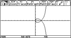
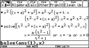
5 The strophoid
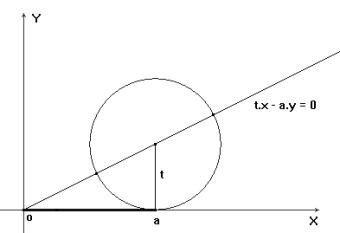
|
Given a line segment with length a. Consider a circle tangent to the line segment in one of its endpoints. Draw a line through the other endpoint and the centre of the circle. The locus of the points of intersection of this line with the circle, by letting vary the circle, is called a strophoid. The locus consists of the points of intersection of the associated curves: the line
and the circle
when choosing the subjoined coordinate system. |
|
|
|
Fig. 8: Dynamic generation of the strophoid |
|
|
|
|
|
Fig.9: Ingredients of the strophoid |
||
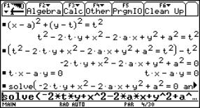
The classical procedure consists of eliminating the parameter t from the system of equations of the associated curves, yielding the cartesian equation of the curve. For students however it is more natural to look for the points of intersection of the associated curves. This gives the parametric equations of the curve. However this often leads to complicated calculations. This is no longer an objection when the calculations are left to a calculator with a CAS.
We enter the equations of the circle and the line and solve for x and y :
|
|
|
|
Fig. 10a |
Fig. 10b |
Since the circle and the line have two points of intersection, we find two solutions connected with "or":
|
|
and |
|
or |
|
and |
|
Now we let draw the curve with these parametric equations for a = 2:
|
|
|
|
Fig. 11: The strophoid – lower part |
|
|
|
|
|
Fig. 12: The strophoid – both parts |
|
By eliminating the parameter t from the system of the associated curves, we expect the cartesian equation of the strophoid.
|
|
|
|
Fig. 13a |
Fig. 13b |
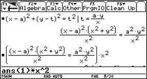
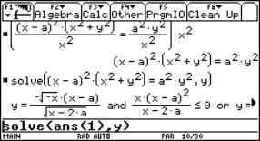
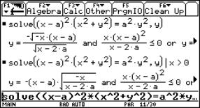
As a wrong result however we obtain the functions
![]()
with as domain the empty set! By imposing the condition x > 0 we do get the correct functions
![]()
yielding the same curve for a = 2 as the parametric representation:
|
|
|
|
Fig. 14a |
Fig. 14b |
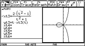
Now we replace x by x+a in the cartesian equation (x–a)2(x2+y2) = a2y2 in order to translate the double point (a,0) of the curve to the origin of the coordinate system. Next we intersect the curve with the line y = t x. We then obtain one parametric representation for the whole strofoid by calculating the coordinates (x, y) of the point of intersection in function of the parameter t. Again we check this with a graph for a = 2:
|
|
|
|
Fig. 15a |
Fig. 15b |
6 Conclusions
Thanks to computer algebra it becomes possible to eliminate parameters directly, without the use of determinants. Through this one can treat the subject elimination at an earlier stage and it has the additional advantage that the meaning of the concept elimination is clarified.
The student can quickly make a graph and see that the parametric and cartesian representations yield the same curve.
The choice of the window and the parameter interval is very important to obtain a nice graph. One needs to take the necessary time to discuss this subject, this provides insight in the geometrical meaning of the parameter.
One can "only" manipulate formulas with "computer algebra". A computer cannot "see" the meaning of a letter in a certain equation. Does this letter represent a constant, a variable or a parameter? What is given en what is asked? What is the set of numbers we are working with? These are essential aspects of algebra (fortunately?) reserved for the human brain.
Consequently, it is not surprising that computer algebra sometimes causes "errors", like
|
|
|
sometimes written as |
|
|
which may lead to functions with a different domain.
The user of a CAS must stay watchful; computer algebra forces us to reflect on manipulating formulas and to state explicitly conditions that are often implicitly assumed when we work with paper and pencil.
Theorema-based TI-92 simulator
for exploratory learning
Youngcook Jun
Hagenberg, Austria
3. How to build Derive simulator with Theorema
4. Exploratory learning with syllogism tasks
One of the Theorema system’s capabilities provides a computional session that enables a developer to simulate an existing graphing calculator such as TI-92. Moreover, the deductive reasoning facility of Theorema allows the simulator to deal with propositional and predicate logic for pedagogical purposes. We present how to apply the use of such a simulator to help students explore mathematical ideas in terms of the blackbox/whitebox principle. This experimental approach is demonstrated with integrated modes of computing, solving and proving. This paper is motivated by how to encourage students to expore his/her own mathematical thinking based on algorithmic and logical operations built into the Theorema system.
1 Introduction
For mathematics learning and teaching, many computer programs are available in schools. Among them, Computer Algebra Systems(CAS) are adopted to help students manipulate algebraic expressions and graphical representations for mathematical objects (Kajler 1998, Karjan 1992). Even though most CASs generate immediate answers for given input expressions as a black box, students are encouraged to focus on manipulating various expressions with different problem contexts so that they can engage in high-level thinking by reducing low-level computational burden (Tall 1991). In this regard, Buchberger suggested how to use CAS for educational purposes in terms of a black box/white box principle (Buchberger 1990). The transition from the use of black box to that of white box can be followed by a creativity cycle that consists of the several steps: 1) work on various examples 2) try to find any patterns out of them to make any conjecture 3) try to verify the conjecture 4) come up with knowledge bases (i.e., theorems) in terms of building algorithms 5) try one of those algorithms as a black box to new examples, and so on. In this paper,it is assumed that exploratory learning takes place in the steps of 1) and 2). During this exploratory learning, students pursue different layers of mathematical ideas with many examples, already earned concepts and algorithms by experimenting and operating concrete math objects in a constructive way.
To investigate this exploratory learning phase more deeply, we try to build a simulator for algebra (Derive) part in TI-92 with Theorema. Theorema is an integrated suite for teaching logic and mathematics with collection of general and special provers (Buchberger e.a. 1997). It can generate automated theorem proofs in a natural language style presented in Mathematica notebooks. Besides the capability of proving, solving and simplifying, Theorema’s language constructs are dealt with mathematical expressions that are similar to the conventional mathematics. With Theorema’s data structure such as tuple notaion , it is relatively easy to manipulate algebraic expressions, logical deduction and theorem proving. For the current work, we only try to simulate Derive part of TI-92 with keyboard layout so that the future version will generate sequences of keystoke maps for various simulated commands. The internal representation of Theorema will deal with keystrokes of a user’s action in particular learning mode such as exploratory learning to capture and verify any emerging patterns in terms of equivalent relations and equality. This direction suggests how to demonstrate integrating CAS and automated deduction for educational purposes as an experimental apparatus.
2 Design principles
The design of this system consists of three parts considering Theorema’s distinct features such as computing, solving ande proving. The computing part is carried out in the computational session while proving part is done in the proving session. The current Theorema does not provide a rich set of solving mechanisms yet. Derivations in each problem solving is seperately designed in this simulator. Derivations are just a collection of intermediate steps without explicit verbalization in a whitebox sense. The reason behind this is that output screen of TI calculator is limited for detailed verbal descriptions for those intermediate steps. How to design such a simulator to mimic the behavior of TI-92 calculator is closely related to Theorema’s capability mainly by integrating its computational and proving session.
Given a fixed set of commands and menu clicks, how to compose different commands to come up with pedagogically meaningful output? This viewpoint concerns the technical aspects of manipulating TI-92 keystrokes to help students attain the level of understanding. As students gradually experiment with algebraic expressions and numbers with possible derivations in certain cases, they probably get into the stage of guessing some properties of the target mathematical objects. Such conjecture making seems to motivate the students to attempt to verify certain properties with proving capability of Theorema as a blackbox. The whitebox part of Theorema can be available as a separate Mathematica notebook. With the help of Theorema’s built-in provers, the students can confirm or disconfirm their conjectures in the simulated screen. This process guides them to make a concrete algorithm with which it can be served as a blackbox to do experiment with other sets of data. Such a process is described in terms of a spiral, called creativity cycle. This view guides us the main aspects of designing TI-92 simulator.
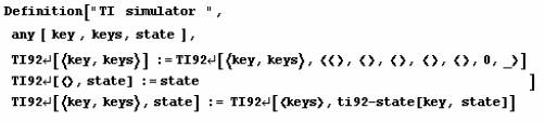
3 How to build Derive simulator with Theorema
In Theorema, the user can define both logical and mathematical definitions with various quantifiers in computational and proving session. Based on Mathematica (Wolfram 1996), Theorema’s logical inferencing mechanism allows users to work on conventional (abstract) and computational (concrete) mathematics. The main part of our simulator is coded by a recursive procedure that feeds an input expression one by one. Each expression triggers one of the “ti92-state” rewriting rules to yield an intermediate state to mimic Derive’s algebraic commands. With this new intermediate state, another input is fed for the next rule match. This evaluation part is carried out in the Theorema’s computational session. The output is written in Mathematica codes for making different box styles with colors to mimic TI-92 screen layout. The current version of the simulator is only close to algebraic manipulation part without a graphics mode. The next sample code illustrates how Theorema’s codes look like for the main part that is based on recursion.
|
|
|
|
|
|
|
|
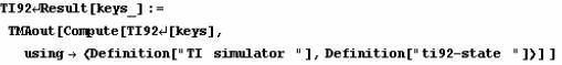
Algebraic manipulation
Most of the content materials tested in this simulator are from written manuals developed by TI and Kutzler (1997). It is noted that some expressions (i.e., equality sign) are not identical with TI-92 expressions. The frame layout is quite elastic since there is no screen layout controller at this point. The whole part of current version covers three directions: numerical, algebraic and logical expression. In Fig 1, various examples are depicted in PC environment. The following code shows how 3 different TI commands (solve, csolve, factor) and 1 built-in Mathematica command (Together) are executed with a simulated screen.
|
|
|
|
|
|
|
|
|
Fig. 1: Theorema’s call for simulated TI commands and output layout |
||
From this prototyping, it turns out that most of the Mathematica’s commands can emulate Derive’s algebraic commands with slight modification. However, some Derive’s commands are not availble in Mathematica. In such a case, it is programmed with Mathematica language as shown, for example, in the case of proper fraction, “propFrac”. It is noted that for the educational purposes, simulated TI commands (eg., solve) only generate real values whereas “csolve” generates complex valued-solutions. Other commands deal with conditional checking with a certain value for a given variable with “|” substitution symbol. This equational checking is also available for experimenting various numerical substitutions for an expression at hand.
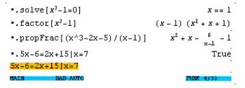
Derivations for equation solving
Equation solving in TI-92 is usually carried out by rewriting terms without showing intermediate steps as a black box. This feature can be modified into a white box considering cognitive fidelities of the students according to different learner levels. In fact, low-level and intermediate level students seemed to prefer following intermediate solving steps (Jun 1995). With TI-92, however, students can manipulate different ways of transforming algebraic rules explicitly by extra work on their own. For example, Kutzler introduced several ways to isolating a target variable to find a solution given a system of linear equations. Our simulator rather directly generates a sequence of algebraic transformation including an answer all at once (see stepSolve). Currently, the number of transformation rules is less than 10 since we try to capture general patterns associated with rewriting rules as minimally as possible (Kajler 1998).
|
|
|
|
|
Fig. 2: Commands for step-by-step algebra rewriting |
||
Propositional calculus with Theorema
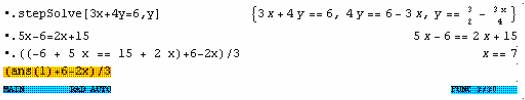
The most distinct feature of our simulator comes from the addition of PredicateProver that is a special prover embedded in Theorema. In this experimental version, we try to connect algebraic manipulation with propositional calculus so that students can go through different representations in school mathematics. Due to the fact that propositional calculus is derived by Boolen logic, students can practice logical inference when a certain property occurs during their work along with a creative cycle. This helps students to make a conjecture considering the fact that such a conjecture might be better represented by predicate calculus. As Theorema generates step-by-step natural language illustration in each step of proving, students can grasp how logical deduction goes without much difficulty. A frontend interface to the simulator send a request for proving to one of the Theorema’s provers to generate verbalized logical explanations in terms of a proof tree (Figure 3). In this way, students can invoke graphing calculator part as well as logical deduction part to explore deep sides of mathematics. The followoing figures presents how propositinal statement is proven in user-friendly interface. The taget task is:.
|
|
|
|
|
|
|
|
Fig. 3: The simulator’s screen and PredicateProver’s step-by-step proof |
|
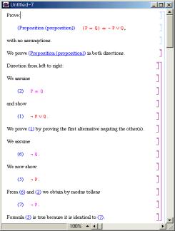
4 Exploratory learning with syllogism tasks
According to Buchberger (1999), the use of Theorema can be applied to theory exploration rather than proving isolated theorems. Considering the fact that secondary mathematics textbooks contain only several dozens of theorems in geometry, proving is not regarded as main mental activities in secondary schools. However, proof training is indispensable for high-level mathematics. This aspect implies the importance of making students be engaged with reasoning tasks. With this motivational thing in mind, we consider traditional logical tasks, called syllogisms. There are three methods to deal with them: diagram-based, equational logic and predicate calculus. All of these methods might be difficult for high school students. However, students can visualize their thinking with diagrams and translate mathematical thinking into algebraic formula. At the end, they can verify their conclusions by implicitly calling PredicateProver available in Theorema system. By reading step-by-step annotations in each proved text, students can understand how each proof is derived.
Compared to expert mathematicians who explore mathematics ideas from scratch to grasp coherent ideas in an integrated way by working with each part (layer) of the whole procedure, students usually tend to follow a trial-and-error approach. In doing so, they can use formulae, diagrams, equations to find meaningful derivations. In this paper, it is assumed that algebraic transformation rules with predicate calculus can lead students to explore various properties as they accumulate algorithmic thinking. For example, a student might want to draw a valid conclusion for the following task: “All philosophers are professor. All professors are logicians.” To tackle with such a task, one may use a Venn Diagram by abstact set notation. Given a statement, “All As are Bs. All Bs are Cs.”, the valid conclusion, “All As are Cs,” might be easily drawn either propositional calculus or a Venn Diagram.
Another interesting method is to transform such syllogism premises into equations. The following equations are those in this case: A*B=A, B*C=B. Then A=A*B=A*B*C=A*C, so we have A*C=A which means All As are Cs. To verify this conclusion, we can call Theorema’s predicate prover by converting two premises into predicate calculus form. As for another task, “All A are B, Some B are not C”, the internal code for checking the conclusion “Some A are not C” looks like in the following way with the result “proved”:
|
|
|
|
|
|
|
|
|
|
|
|
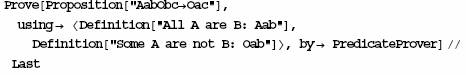
The main prover, called PredicateProver, usually starts with negating the conclusion to find any occurred contradiction. In some cases, the prover produces “failed” result, which means the conclusion can not be proved. Also notice that there are several syllogisms that do not have valid conclusions. In those syllogisms, it is rather difficult for students to encode two premises in a correct way to draw any conclusion. In such cases multiple representations are very helpful to assist their thinking. In syllogism tasks, there are two ways of represent syllogisms: equational logic and Venn diagram. For the first representation, syllogisms are represented in algebraic forms just like high school algebra solving. The simulator part can also produce step-by-step solutions using equational rewriting method. Another representation,.Venn diagram, requires rather sophiscated implementation details that execute conversion process from a Venn diagram to algebraic equations and vice versa. The implementation of this Venn diagram conversion process is left as part of logico-graphic feature available in the future version of Mathematica.
With versitile features available from TI92 simulator, it is then up to students who can touch upon several layers of math contents to investigate any meaningful properties with several provers embedded in the Theorema. In this way, computer algebra in TI-92 can be combined with Theorema’s solving and proving functionality to promote students’ explarotary learning. The overall demonstration of this simulator indicates future work to enhance several things including interface, algebraic expressions, interactive solving with feedback and meta-rules for invoking Theorema’s several provers.
5 Conclusion
This paper illustrates how the combiniation of computer algebra system and automated deduction system can be applied for pedagogical purposes. With the assumption that secondary mathematics learning can be directed to student-oriented exploratory learning instead of passive learning, it is the aim of this study to design and develop TI-92 simulator that can mimic TI graphics calculator based on Mathematica and Theorema. Even though computing and solving is dominant in most parts of secondary school mathematics, the current trend of using CAS suggests various ways of utilizing it to promote students to engage herself/himself in more conceptual levels of mathematical thinking. Theorema’s computational and proving capability has shown that how TI calculators can be implemented for pedagogical purpose with research-oriented CAS such as Mathematica and Theorema. The future study will deal with verification method that ensure pedagogically and logically sound ground in each problem solving step. The emphasis of exporatory learning cast in this paper only suggests how each student can pursue his/her own ideas along with a creative cycle in an intergrated environment of CAS and automated deduction system.
There are two things that need reflective thoughts for the use of CAS and automated deduction for pedagogical purposes layed out in this paper. First, characteristics of students’ exploratory learning might be different compared of mathematician’s exploratory style. More detailed analysis of student-centered exploratory activities are required. This aspect might shed light on how to design CAS with possible use of automated deduction for school mathematics. The second point reflects which equivalent commands or methods are directly appealing to students’ exploratory learning. For example as shown
|
|
|
|
the propositional statement can be checked with truth tables available in TI-92 calculator for school mathematics even though TI-92 simulator can provide predicate calculus styles. From students’ perspective, it seems very important for them to select the most appealing commands out of equivalent classes given a comand or method.
Acknowledgements
This work has been carried out in the frame of the Theorema project at the RISC institute, supported by the "Spezialforschungsbereich for Numerical and Symbolic Scientific Computing" (SFB F013) at the University of Linz. I thank Dr. Bruno Buchberger who helped me to prepare this paper.
References
Buchberger, B. (1990). Should students learn integration rules? ACM SIGSAM Bull.(24), 10-17.
Buchberger, B. (1999). Theory exploration versus theorem proving. Mathematica Notebook for the invited talk at the Calculemus Meeting, Trento 1999.
Buchberger, B., Jebelean, T., Kriftner, F., Marin, M., Tomuta, E. ,& Vasaru, D.(1997). A Survey of the Theorema Project. W. Kuechlin (ed) Proceedings of ISSAC'97. ACM Press, 384-391.
Jun, Y. (1995). Learning how to solve linear equations by teaching the computer: Development and formative evaluation. Unpublished doctoral dissertation, University of Illinois at Urbana-Champaign.
Kajler, N. (Ed.) (1998). Computer-Human Interaction in Symbolic Computation. Springer, Wien.
Karian, Z. (Ed.) (1992). Symbolic computation in undergraduate mathematics education. MAA Notes 24, Math. Ass. of America.
Kutzler, B. (1997). Introduction to the TI-92. bk teacheware.
Tall, D. (Ed.) (1991). Advanced mathematical thinking. Kluwer
Wolfram, S. (1996). The Mathematica Book. Wolfram Media and Cambridge University Press.
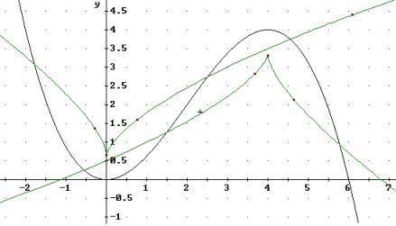
Krümmung als Grenzwert - Curvature as limit
Karl-Heinz Keunecke
Kiel, Germany
1. Das Unterrichtskonzept - The didactical concept
2. Realisierung der UE mit Derive - Realisation of the teaching unit with Derive
1 Das Unterrichtskonzept - The didactical concept
 Über „Gefährliche Kurve” aus dem Strassenverkehr gewinnt man schnell den
Einstieg in das Thema. Ein Auto, das eine Kurve durchfährt, darf diese nicht
schneiden, sondern hat sie nur zu „berühren”. Für die kurze Zeit, in der der
Einschlag des Steuerrades nicht geändert wird, bewegt sich der Wagen auf einem
Kreisbogen. Damit sind bereits alle Begriffe zur Verfügung gestellt, die benötigt
werden, um mit Hilfe des Radius des Krümmungskreises r bzw. durch k = 1/r ein Mass für die Krümmung eines
Funktionsgraphen zu definieren.
Über „Gefährliche Kurve” aus dem Strassenverkehr gewinnt man schnell den
Einstieg in das Thema. Ein Auto, das eine Kurve durchfährt, darf diese nicht
schneiden, sondern hat sie nur zu „berühren”. Für die kurze Zeit, in der der
Einschlag des Steuerrades nicht geändert wird, bewegt sich der Wagen auf einem
Kreisbogen. Damit sind bereits alle Begriffe zur Verfügung gestellt, die benötigt
werden, um mit Hilfe des Radius des Krümmungskreises r bzw. durch k = 1/r ein Mass für die Krümmung eines
Funktionsgraphen zu definieren.
Um mit Schülerinnen und Schülern den Krümmungskreis zu konstruieren, geht man am besten zunächst von einem Kreis aus, bei dem der Mittelpunkt als gemeinsamer Schnittpunkt aller Normalen gegeben ist. Der Krümmungskreis ist hier überall gleich und mit dem Funktionsgraphen identisch. Die Methode der Konstruktion des Mittelpunktes des Krümmungskreises durch die Schnittpunkte von Kurvennormalen lässt sich auch auf beliebige Funktion übertragen. Dies wird mit Fig.1 erläutert.
A road sign "Dangerous curve" can introduce to the problem. A car driving through a curve must not "cut" but osculate the road. For a short while when the steering wheel is in a certain position the car moves on an arc of a circle. From this discussion all the expressions are available to define the curvature of a function by means of the radius r of the osculating circle as k = 1/r.
We try to find a circle, which osculates the given graph in A (5; f(5)). Starting with the normal line of graph f in A we find neighbouring normals for xi = 6, 5.75, 5.5, 5.25 and their intersection points with the normal line for x = 5. x4 = 5.25 leads to centre M4 and this circle seems to be at least a good approximation for the desired circle. (Figure 1)
|
|
|
|
|
|
Fig.: 1 |
|
Es soll ein Kreis gefunden werden, der den Funktionsgraphen an der Stelle x = 5 berührt. Dazu wird zunächst in dem Punkt A(5; f(5)) die Normale zu dem Graphen von f und anschließend werden weitere Normale an den Stellen 5,25; 5,5; 5,75 und 6 gezeichnet. Die Schnittpunkte mit der Normalen durch A sind M1 bis M4. Nun werden Kreise um die Punkte M1 bis M4 jeweils durch den Punkt A gezeichnet. Während die Kreise mit r1 und r2 den Graphen noch mehrfach schneiden, so scheint der Kreis mit r4 bereits etwa die gewünschte Eigenschaft zu haben. Man wird vermuten, dass die Näherung umso besser wird, je dichter die Normalen an die feste Normale durch A heranrücken. Hieraus kann nun im Unterricht eine Strategie für das weitere Vorgehen entwickelt werden.
1 Gleichung für die Normalen an den Stellen a und a + h aufstellen.
2 Schnittpunkt dieser beiden Normalen bestimmen.
3 Untersuchen, ob es einen Grenzwert der Punktfolge für h ® 0 gibt.
4 Falls die Folge konvergiert, den Radius des Krümmungskreises und die Krümmung berechnen.
1. Find the equations of the perpendicular lines on places a and a + h.
2. Calculate the intersection points.
3. Investigate if there is a limit for the sequence of the intersection points for h ® 0.
4. In case of convergence calculate the radius of the osculating circle and its reciprocal value - the curvature.
First we will investigate the curvature of given functions to proceed in generalizing the procedure to obtain the well-known formulae for the radius of the osculating circle and the curvature.
Mit diesem Konzept wird zunächst die Krümmung gegebener Funktionen an vorgegebenen Stellen mit Hilfe von Grenzprozessen untersucht. Das Verfahren lässt sich aber auch auf eine beliebige Funktion f(x) und die Stelle x = a anwenden. Dann gewinnt man die bekannten Formeln für Krümmung und Krümmungskreis, die schließlich zur Bearbeitung praktischer Probleme genutzt werden.
2 Realisierung der UE mit Derive - Realisation of the teaching unit with Derive
Bei Benutzung von Derive5 kann jeder Schüler ein eigenes Arbeitsblatt anlegen, in dem alle Definitionen und Befehle individuell kommentiert werden können. Außerdem kann jede Graphik in dieses Worksheet eingebunden werden. Es ist also im Grunde keine zusätzliche Mitschrift in einem Heft erforderlich, denn der Ausdruck des entsprechenden dfw-Files liefert alle erforderlichen Informationen einschließlich der Hausaufgaben mit den Lösungen.
|
|
Fig. 2: Derived from expression #4
Fig. 3: Derived from expression #7 |
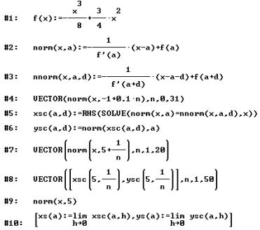
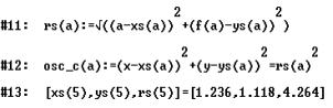
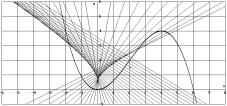
Leider wird beim Aufruf von norm(x,a+h) im allgemeinen Fall der Term f'(a+h) nur als f'(a) ausgewertet. Daher ist für die benachbarte Normale eine zweite Funktion nnorm(x,a,d) notwendig. Die Berechnung der Koordinaten des Schnittpunktes erfolgt in den Zeilen #5 und #6. In #11 wird der Radius des Krümmungskreises ermittelt. Die Ergebnisse an der Stelle x = 5 finden sich anschließend.
Zunächst erhalten die Schülerinnen und Schüler mit Zeilen 1 und 2 die Möglichkeit, zum Graphen der Funktion f die Normalen zu konstruieren. Damit können sie die Lage der Schnittpunkte der Normalen zu untersuchen. Eine Normalenschar wird z.B. mit Zeile #4 erzeugt, die in Fig.2 dargestellt wird.
Darin kann aus den Schnittpunkten benachbarter Normalen auf die ungefähre Lage der Mittelpunkte der Krümmungskreise und deren Radien geschlossen werden. Die zugehörige Krümmung ist im Nullpunkt am größten und bei x = 2 hat sie den Wert 0, da hier die Normalen parallel verlaufen.
Um die Schnittpunkte algebraisch zu bestimmen wird die Gleichung
norm(x,a) = nnorm(x,a,d) für d ¹ 0
in #5 gelöst und in #6 der zugehörige y-Wert berechnet.
|
Mit d = 1/n werden in #7 für a = 5 und für n = 1,...,20 die zugehörigen Normalen berechnet. Aus der graphischen Darstellung in Fig.3 kann man vermuten, dass die Schnittpunkte der Normalenschar mit der Normalen an der Stelle a = 5 einem Grenzwert zustreben. Dies erkennt man noch deutlicher, indem man für die gleichen Bedingungen nur die Punktfolge
einzeichnet, wie es in Fig.4 geschehen ist. |
|
|
Fig. 4 |
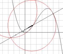
Als nächster Schritt sind nun die Grenzwerte für xsc(a,d) und ysc(a,d) zu berechnen (#10) Man erhält:
(xs; ys) » (1.237; 1.118)
Aus dem Abstand dieses Punktes von A errechnet man (#11) den Radius des Krümmungskreises rs » 4.265. In #12 wird die Gleichung des Krümmungskreises als Funktion von a festgelegt. Er ist in Fig.4 eingezeichnet worden und ist somit ein für Schülerinnen und Schüler wichtiger Nachweis, dass die durchgeführten Berechnungen richtig sind.
Unfortunately f'(a+h) doesn´t evaluate in an expression using a generic function f(x) correctly. It appears as f`(a). That is the reason that nnorm(x,a,d) must be defined The intersection point is calculated in #5 and #6, the radius of the circle is result of #11.
The students are encouraged to produce a family of perpendicular lines (expr #4, Figure 2). Using a sequence for h (e.g. k = 1/n) with a = 5 they create a family of perpendicular lines approaching the normal line in a = 5.(expr #7, Figure 3) They can estimate the position of the "last" intersection point and confirm their conjectures by evaluating and plotting the sequence of points in #8 (Figure 4). The next step is performing the limit process in #10, observing the convergence, followed by calculating the radius of the osculating circle (#11). #12 generates the osculating circle as a function of a.
The sequence of points may be divergent. Approaching a = 2 using norm(x,2+h) or creating a point list similar to that given in #7 results in infinite large numbers. The students should discover that in a point of inflection the radius of the osculating circle is infinite, thus curvature is 0.
Having worked out sufficient examples one can proceed generalizing the problem. Working with a generic function f(x) and an arbitrary position a delivers results in # 20 and #21 immediately.
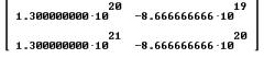 Nicht immer sind die entstehenden
Punktfolgen konvergent. Nähert man der Normalen im Wendepunkt a = 2 eine Normale nnorm(x,2+h) immer mehr an, so entfernt sich der
Schnittpunkt der beiden Normalen immer mehr. Das ist bereits aus Fig.3 zu
vermuten, weil an dieser Stelle die Normalen offensichtlich parallel verlaufen.
Nicht immer sind die entstehenden
Punktfolgen konvergent. Nähert man der Normalen im Wendepunkt a = 2 eine Normale nnorm(x,2+h) immer mehr an, so entfernt sich der
Schnittpunkt der beiden Normalen immer mehr. Das ist bereits aus Fig.3 zu
vermuten, weil an dieser Stelle die Normalen offensichtlich parallel verlaufen.
Eine Punktliste ähnlich #8 mit a = 2 anstelle von a = 5 - womöglich mit einer stärker konvergierenden Folge für k - ist ein deutlicher Hinweis auf die Divergenz.
Wenn eine ausreichende Anzahl von Beispielen im Unterricht bearbeitet worden ist, dann kann die Bestimmung der Krümmung für eine beliebige Funktion f an der Stelle a nach der gleichen Methode durchgeführt werden. Dies wird anschließend gezeigt.
Von diesen Lösungstermen sind nun die Grenzwerte für h ® 0 zu berechnen. Das leistet Derive ebenso wie viele andere CAS (Keunecke 2000) nicht. Bekanntlich sind diese Terme so umzuformen, dass die Differenzenquotienten von f und f' auftreten, deren Grenzwerte dann f' und f'' sind. Der folgende Term zeigt nochmals die Rechnerlösungen für xsc(a,h) und ysc(a,h).
|
|
|
|
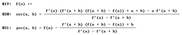
Daraus erhält man nach der beschriebenen Umformung für die x-Koordinate:
Derive (and other CAS) are unable to discover the derivatives in these expressions - so rediscover your pre-Derive manipulating skills to rewrite expr #20 and #21 to calculate the limits leading to the centre coordinates of the circle and its radius - the last step can be done supported by Derive:
|
|
|
|
Der Grenzwert ist dann:
|
|
|
|
Für die zugehörige Ordinate erhält man
|
|
|
|
und für die Krümmung
|
|
|
|
Für diese Rechnungen kann man bereits wieder das CAS verwenden.
|
|
|
|
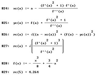
Literatur
Keunecke, K.-H. (2000) Behandlung der Begriffe Folge, Grenzwert und Ableitung am Beispiel der Krümmung. Prax. Math. 5/42.
Mathematics with graphic and symbolic calculators – Teacher training in Lower Saxony
Heiko Knechtel
Bückeburg, Germany
3. T³-Regional conferences in Germany
4. Contents of teacher training
History - organisation - contents of teacher training in Lower Saxony: In Lower Saxony, Germany, a new concept of teacher training was developed from the mathematics advisers: Every math-teacher at high school has to take part in 4 math workshops within 3 years. They should learn, how to integrate the new technology of the hand-held calculators and dynamic geometry in their own math lessons.
Interested teachers were trained within 2 years for math-multipliers. The math-multiplier-groups were divided in teams of two persons. Each team is responsible for six schools in their region. Each team focussing on special interests for each school and go ahead for four times with the groups. They will visit the colleagues in their own school and give several workshops there. Items of the workshots are handling with graphic and symbolic calculators and dynamic geometry; developing units with the new technology basing on their traditional math lessons by their own. After testing their own units during half a year the last 2 workshops give them a view on new possibilities in math lessons, especially in advanced or real-world mathematics. Supplementary every year in each region there are regional T3-conferences with a main lecture and up to 15 workshops over the day.
1 History
Since the beginning of the nineties there was a great discussion in Germany about the influence of handheld technology in mathematic education. In 1992 there were the first workshops about graphic calculators in math lessons, specially in Calculus, all over in Lower Saxony. The teachers were very reserved facing the new technology. Several great national conferences about the influence of symbolic calculators in math lessons followed, all emphasize the importance of computer
algebra systems in teaching and research mathematics. But the reservation of the teachers didn't move. Only a few teachers all over Germany tried to integrate the new technology in their math education.
With the development of the new symbolic handheld calculator TI 92, there was a first change in the math lessons at the highschools: several students heard about the new technology and wanted to test it, a revolution from the ground seemed to be started, but the German teachers still didn't want to change their math education.
2 Organisation
In the year 1997 I started a new attempt together with thirty very interested teachers in the region of Hanover. These teachers were trained for "math‑multipliers”. For a time of fourteen days we had several workshops with the new technology like in the summer university in Ohio and we started to developed new math units for the employment of handheld technology. After one and a halve year the teachers were ready to show their colleagues at school an interesting new math concept. The government of Lower Saxony promised to promote the teacher training for several years. The new concept of teacher-training was developed from the mathematics advisers:
Every math‑teacher
at highschool should take part in 4 math workshops within three years. they
should learn, how to integrate the new technology of the handheld calculators
in their own math lessons.
The
“math-multiplier”-groups were divided in teams of two persons. Each team is
responsible for six schools in their region. Each team focussing on special
interests for each school and go ahead for four times with the groups. They
will visit the colleagues in their own school and give several workshops there.
In the first
workshop the teachers were introduced in the handling of graphing and symbolic
calculators and dynamic geometry systems like Cabri Geometre, Euklid or
Cinderella.
In the
second workshop they will develop units with the new technology basing on their
traditional math lessons by their own ("learning by doing").
The last two
workshops will start half a year later. In the meantime the teacher should test
their own units. The last workshops give them a view on new possibilities in
math lessons, specially in advanced or real‑world mathematics.
The teacher should learn new contents of mathematic lessons, new lessons with old contents and they should learn new ways of math teaching and learning. They should learn, how students can explore the mathematics by their own .
3 T³-Regional conferences in Germany
In the last three years all over Germany there increase local Regional-Conferences. The idea is, to give teachers on the one side an overview of the potentialities of fully integrated technology in the classroom and on the other side to give them the chance to experience with handheld-technology. Therefore the structure of the conferences is orientated at a central lecture and several workshops.
Organization:
Cooperation between university – government –
local high schools in the region
1 lecture of
a professor of mathematical didactic
several workshops about topics of school-mathematics
period of one day at the weekend,
sponsored by
T³-Europe in cooperation with a local organisation-team
4 Contents of teacher training
Example 1 “Cubic splines – a real world model in math lessons”
|
|
|
|
|
Fig. 1: Surface modelled by splines |
|
Fig. 2: Cross-section modelled by splines |
The spline interpolation is an excellent method, to describe some real world problems. In many industries, e.g., shipbuilding, automotive and aircraft, the final full or nearly full size shape is determined by a process called lofting. In the shipbuilding industry it is necessary to determine the shape of the ship with more accuracy than it is possible on a small paper drawing. Therefor it is common practice to redraw the ship´s lines at full or nearly full size on a large wooden floor located in the “mold loft”. The skilled craftsman who perform this task are known as “loftsman” and the process as “lofting”. With the developement of mathematical tools (in Geometry and Computeralgebra) there was considerable interest in developing a mathematical model of this process. As a result, the mathematical spline is derived from its physical counterpart – the loftsman spline. A physical spline is a long narrow strip of wood or plastic used to fit curves through specified data points. The splines are shaped by lead weights called “ducks” , in German “noses”. By varying the numbers and position of the lead weights the spline is made to pass through the specified data such that the resulting curve appears “smooth” or “pleasing to the eye”.
Considering the physical spline as a thin elastic beam, the shape of the beam is obtained from the Euler´s equation for the bending moment along the length of the beam. With several ideas you can prove, that the spline is a piecewise poynomial of degree 3.
Because not all students and not all teachers are physicans it is very problematically to teach them the idea of splines in this way. Better is the visualisation of the idea. Take five digital points, ask for the interpolation polynomial and show, that there is a better one, which smooth the optimal shape. You need a model, which can realize the two interpolation functions.
|
|
|
|
Fig. 3 |
Fig. 4 |
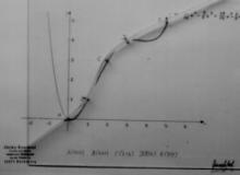
If you have to construct a location route of an high speed train or a shape of a ship there are the following steps:
survey the scenery and determine some special
points
transfer the points on a digital model
try to calculate a interpolation function
control the model
revise the model
control the revised model
translate the model back to reality and control
Boundary conditions for spline-functions :
spline is an interpolation function
piecewise polynomial of the degree 3
continuous first and second derivatives
the continuation at the beginning and the end of
the spline is linear
The four boundary conditions for a spline with 5 data points A, B, C, D, E are as follows:
|
1. |
|
spline is an interpolation function |
|
2. |
|
equal slope on both side of the points |
|
3. |
|
equal 2. derivative on both sides of the points |
|
4. |
|
the continuation of the spline is linear |
With these terms you get an system of linear equations concerning to the coefficients of the 4 cubic splines. The degree of the system is 16, the solution with the TI-92 take not much pain. Because the students have not to calculate by hand they interpretate the solution without emotions. They can compare the polynomial and the cubic spline withe their graphic calculator. Finally they can variate the problem: If one of the points is variable, what is then the reaction to the cubic spline?
|
|
|
|
|
|
|
|
Fig. 5: Polynomial interpolation |
Fig. 6: Interpolation by spline |
Example 2: “The world-pop-clock – from the linear model to the logistic model”
Population‑ projections first became important to political philosophers in the late eighteenth century. As concern for scarce resource has grown, so has interest in accurate population projections. There are several models of population growth, discrete and continuous models. They all used to model human and animal population growth as well as growth processing in economics.
World POPClock Projection: According to the International Programs Center, U.S. Bureau of the Census, the total population of the World, projected to 2/23/00 at 12:36:58 GMT (2/23/00 at 7:36:58 AM EST) is 6,046,287,932
![]()
Monthly World population Figures:
07/01/99 5,996,708,634
08/01/99 6,003,179,337
09/01/99 6,009,650,041
10/01/99 6,015,912,012
 11/01/99 6,022,382,716
12/01/99 6,028,644,688
01/01/00 6,035,115,391
02/01/00 6,041,586,095
03/01/00 6,047,639,334
04/01/00 6,054,110,038
05/01/00 6,060,372,009
06/01/00 6,066,842,713
07/01/00 6,073,104,685
![]()
Discrete models of population growth
Applications with the data/matrix‑editor and recursive defined sequences
1. The linear model ‑ the absolute growth rate is constant
|
|
un+1 = un + c , c = const. |
|
|
|
uo = ustart |
|
|
|
un+1 ‑ un = c |
absolute growth rate |
2. The percentage model ‑ the relative growth rate is constant
|
|
un+1 = un + c×un = (1 + c)×un |
|
|
|
uo = ustart |
|
|
|
|
relative growth rate |
3. The exponential model (continuous growth) ‑ the relative growth rate is constant
The simplest model for population growth is to assume that the relative growth rate is constant. Because there is a continuous growth you get a differential equation:
|
|
|
|
|
|
|
relative growth rate |
|
|
|
|
|
|
|
P0 is the population when t = 0 |
4. The logistic model ‑ the relative growth rate is a linear decreasing function of P
|
discrete: |
|
|
|
continuous : |
|
|
|
|
|
L limit of the population |
|
|
|
general logistic equation |
|
|
|
formula for the logistic curve |
|
|
|
|
Explorations with the TI-92
|
|
|
|
Fig. 7a |
Fig. 7b |
|
|
|
|
Fig. 7c |
Fig. 7d |
|
|
|
|
Fig. 7e |
Fig. 7f |
|
|
|
|
Fig. 7g |
Fig. 7h |
|
|
|
|
Fig. 7i |
Fig. 7j |
Example 3: “The flighty ribbon – DGS connected with calculus and linear algebra”
You move a stone connected with a ribbon nearly without mass on a parabolic curve. The problem: What is the curve of the flighty ribbon? With Dynamic Geometry Cabri on the TI-92: You define a parabolic as the curve of all points, which has the same distance to a line and a Point F. The flighty ribbon is the tangent in the curve-point with a determinate length.
|
|
|
|
|
|
|
Fig. 8 a-d: The curve of the endpoint of the flighty ribbon |
|
The equation of the parametric curve:
The function of the stone trajectory: y = -a×x². The parametric function is:
|
|
|
|
The flighty ribbon is the tangent of a constant length L . If we try to calculate this with the help of the analytical Geometry we find the vector Fl(t):
|
|
|
|

with k describing the constant length of the ribbon.
As a parametric function:
|
|
|
|
With this parametric function you can analyse special problems:
|
|
|
|
|
Fig. 9: The curve with variable ribbon length |
|
|
|
|
|
Fig. 10: Curve with variably open parabola |

What
is the curve of the peaks of the flighty ribbon, if the length is variable?
Zeros of the y-derivative of the parametric function:
|
|
|
and |
|
with t³0 |
|
|
|
with t³0 |
|
|
|
|
|
Fig. 11: The curve H(x) of peaks |
In special cases of the length of the ribbon or
the opening of the parabolic you get points with a vertical tangent.
Calculating the „vertical points“ with the x-derivative:
|
|
|
giving the zeros: |
|
|
|
|
In combination (substitute L in FL(t)) with the function FL(t) you get: |
|||
|
|
|
for t£0 |
|
|
|
Fig. 12: The curve S(t) of vertical points |
||
Standardizing the normal probability distribution - An anachronism?!
Josef Lechner
Amstetten, Austria
1. Normal distribution and standard normal distribution
2. What are the reasons for this anachronism?
3. Advantages of the new approach
Numerical calculators have replaced all function tables (like tables for sin, cos, tan, ln, lg and so on) from textbooks and classrooms. Nowadays there is only one exception remaining: tables for the standard normal probability distribution (i.e. normal distribution with mean 0 and variance 1) can be found in every student textbook used in statistic courses. What are the reasons for this anachronism? Are there traditional or technical reasons or is it something else? What does it mean if the more or less time consuming process of scale transformation can be skipped?
Almost every pupil on the Austrian upper secondary level is faced with the normal distribution in statistics courses, because of its frequent occurrence and its importance within inferential statistics. Dealing with the normal distribution is the only remaining topic where function tables are used. The following pages are to demonstrate that this is a real anachronism.
1 Normal distribution and standard normal distribution
Mathematical modelling and exactification of the empiric fact that continuous random variables are often distributed around its mean in a bell-shaped manner yield to normal distribution. This probability distribution can be described by its density function
Its graph is called Gaussian curve or normal curve. Its maximum shows with the mean m, its inflection points coincide with standard deviation s. By building the integral of this function from -¥ to x you get the distribution function of the normal distribution. It represents the area under the curve of N(x, m, s).
To determine probabilities P(x1 £ X £ x2), it is necessary to calculate the integral of the density function within a certain interval.
|
|
|
|
|
Fig. 1: Normal density function, distribution function and probability in interval [x1, x2] |
||
|
Here all the difficulties start. This integral can only be found by means of approximation. The usual way is to use the so-called standard normal distribution (with mean 0 and variance 1). This can always be achieved by scale transformation. By performing this scale transformation you get the well-known transformation formulas
|
|
|||||
|
Fig. 2: z-transformation |
In this case the function F(z) is the distribution function of the normal probability distribution and represents the value of the integral
|
|
|
|
(This integral is called Gaussian error integral or Gaussian error function.) Its values are listed in tables, which are looked up after scale transformation is made. Afterwards it is necessary to perform back-transformation. To solve examples of this kind, lots of transformation work has to be done. The reader can find numerous little theorems in school textbooks for doing this work. In courses without any technology-support it is necessary to follow such methods – in the same way, as you have to use tables for calculating examples with functions from trigonometry or logarithm functions. Using CAS, CAS-calculators or just powerful numerical calculators you can do calculations without any use of standardisation. Normally you have commands at your hand, which represent density and distribution functions for the normal distribution.
|
Tool |
Density function |
Distribution function |
Probability in interval [x1,x2] |
|
Derive |
definable |
NORMAL(x,m,s) |
P(x1,x2,m,s):= NORMAL(x2,m,s)-NORMAL(x1,m,s) |
|
TI-89 |
TISTAT.NORMPDF(x,m,s) |
TISTAT.NORMCDF(-¥,x,m,s) |
TISTAT.NORMCDF(x1,x2,m,s) |
|
TI-92 Plus |
TISTAT.NORMPDF(x,m,s) |
TISTAT.NORMCDF(-¥,x,m,s) |
TISTAT.NORMCDF(x1,x2,m,s) |
|
TI-92 |
Definable |
definable by approximation |
definable by approximation |
|
TI-83-Plus |
NORMALPDF(x,m,s) |
NORMALCDF(-¥,x,m,s) |
NORMALCDF(x1,x2,m,s) |
|
TI-Interactive |
NORMALPDF(x,m,s) |
NORMALCDF(-¥,x,m,s) |
NORMALCDF(x1,x2,m,s) |
By dealing with normal probability distribution you usually encounter the following basic calculation problems:
|
(a) Calculation of a, g |
(b) Calculation of x, |
(c) Calculation of Î, |
|
(d) Calculation of m, |
(e) Calculation of s |
|
The following example shows a typical set of such problems.
Example: A Viennese manufacturer of wafers filled with hazelnut cream produces sachets of such wafers. The weight of such a sachet is normally distributed with an average of 408 grams and a standard deviation of 12grams.
a1) Which percentage of the sachets weighs at least 400g?
a2) Which percentage of the sachets weighs between 395g and 405g?
b) What do the lightest 20% of the sachets weigh?
c) In which interval of weight are 90% of the sachets?
d) The manufacturer wants to give a guarantee, that 95% of the sachets weigh at least 400g. What must the average weigh then be?
e) The manufacturer is not satisfied with his filling machine. He wants to buy a new one with a smaller standard deviation. He requires that if average is 408g at least 95% of the packets must weigh at least 400g. What will the standard deviation have to be?
Calculating part e) of the above example by using a CAS-calculator like the TI-92-Plus for consists of two steps: Firstly to state the general equation normcdf(x1,x2,m,s) = P and to key in all known values and secondly to call up the remaining variable.
|
|
|
|
Fig. 3 |
|
In order to obtain a representation of the Gaussian bell-shape curve, it is necessary to define the density function (which is also available as command TISTAT.NORMPDF(x,m,s) within the statistics packet). Simple probability examples can be solved in the graphic screen directly (but only approximately).
|
|
|
|
Fig. 4: Approximate solution for probabilities on the graphic screen |
|
Hint: The complete example done by different tools is on www.acdca.ac.at
2 What are the reasons for this anachronism?
Standardisation can only be skipped in school lessons, when a suitable tool is permanently at hand. A numerical calculator, with an implemented density function of the normal distribution – like NORMALCDF(x1,x2,m,s) - is sufficient. It is not necessary to have any CAS, but if you have one at hand, it is as easier. Nevertheless all statistics courses usually use the way of standardisation even if they are supported by such calculators or CAS. What are the reasons for this situation? I think there are a couple of factors that play a role.
Lack of handling knowledge
New users often have a very poor knowledge of the possibilities and the capacity of their calculation tools. So it is not possible to use commands in an efficient way. Moreover they are afraid that it would not be possible to solve all calculation problems concerning normal distribution. Slight difficulties, which could be solved by setting boundaries correctly for mean or standard deviation (which can only be a positive real number) are sometimes a reason to lapse back into the conventional solving method.
Technical problems
By developing the TI-92, TI-92-Plus and the TI-89 an implementation of a normal distribution function has – unfortunately – not been considered. Concerning the TI-92-Plus and the TI-89 this is not a real problem. Every user can download the statistics package TISTATLE.9XK (Flash-Application) into his / her calculator. Hopefully the next update of the operating system has such a function implemented in its standard function catalogue. But a problem remains with the widespread TI-92. Of course you can buy a Plus module to make TI-92-Plus out of it. Otherwise it is necessary to develop an approximation function, which can be given to pupils for their disposal.
Teaching traditions and the domination of textbooks
The biggest obstacle - in my opinion - is our teaching tradition, which is based on standardisation whenever normal distribution is dealt with. In every general statistics course standardisation is taught, in every statistics textbook standardisation is the core of all calculations concerning normal distribution and so this concept remains. Moreover there are some suspicions that this concept doesn’t keep in more sophisticated examples dealing with estimating of parameters or testing examples (which is not the case). Most teachers’ teaching preparations are based on textbooks. They don’t want to deviate too much from the textbooks.
3 Advantages of the new approach
Is doing without standardisation any advantage?
First of all doing without standardisation means skipping a lot of transformation procedures, which are not of any importance for understanding of concepts. Subordinate calculations wouldn’t be necessary. There is more time and room for explorations of normally distributed random variables, for the examination of binomially distributed random variables with great samples and analysing problems concerning the estimation of parameters or testing them.
Are there any experiences using this concept?
In the last years I have tried three times to hold a statistics course without using standardisation (twice using Derive, once using the TI-92 and TI-92-Plus respectively). Experiences have been quite encouraging. It was a little bit tiring with the TI-92 (because of sometimes waiting for results). There were not any problems with Derive or TI-92-Plus.
Using a CAS to teach algebra -
Going beyond the manipulations
Carl Leinbach
Gettysburg, USA
2. Some basic ideas and the division algorithm
3. A student's excursion into pure mathematics - Elementary ideal theory
4. The Remainder Theorem, polynomial expansion, and tangent lines
5. Application - Finding a smooth flight path
In this paper I will examine two of the basic theorems from a first year algebra class, the Division Algorithm and its corollary, the Remainder Theorem for polynomials. These two theorems are the basis of much of the teaching and learning in a first course in algebra. Unfortunately, most of the student’s efforts are devoted to factoring polynomials and finding their roots with little gained in terms of insight as to why they are performing these tasks. In this paper we will show how we can use these theorems to write expansions of polynomials about x=a for a¹0. Once this is done, students can learn about the idea of local linearity and tangent lines to the graphs of polynomials. I will mention two applications of these ideas. One is an application to pure mathematics; the other is to a more real world setting.
1 Introduction
One of the mantras of those instructors who advocate the use of CAS in the teaching of mathematics is: "Technology and the CAS allow us to teach students mathematical concepts, not just mathematical manipulations." The belief is that the use of Computer Algebra, Graphic, and Numerical Calculation software or calculators frees the student from the distraction of messy, and now meaningless, manipulations to concentrate on how particular concepts are applied to mathematical problem solving situations.
Josef Böhm in his wonderful lecture, "A Plea for Pure Mathematics" given at the Third International Derive and TI-92 Conference in 1998, talked of another use of the CAS for learning and teaching mathematics. This use also eliminated the distraction of tedious calculations. In this case the students were exploring the meaning and properties of the mathematical idea of least common multiple and greatest common divisor. They used the mathematical definition as a springboard for their investigations into an adventure in elementary number theory. A very interesting fact is that Böhm was working with students in a vocational school. The CAS was used to capture their imagination, curiosity, and creativity.
This paper presents a blend of the two ideas. It starts with the extension of the idea of polynomial division and using a program written by the author in Derive5® to factor polynomials, finds the greatest common divisor of two polynomials. In the hands of a creative teacher, such as Böhm, this idea can be carried into an adventure in elementary ideal theory. Another direction for the use of this idea is to generate applications.
In short, we will use the CAS as a partner in a legitimate mathematical investigation that can be conducted with students who are only at the early stages of their mathematical development. The hope is that mathematics will become an exciting and vital subject that they may wish to pursue. The CAS provides the opportunity. The instructor's appropriate use of the tool provides the inspiration.
2 Some basic ideas and the division algorithm
We begin with two basic ideas. The first is the idea of the degree of a polynomial, and the second is that of the leading coefficient. Neither Derive5, nor the TI-89/92+ have built in routines that will compute these quantities. However, it is relatively easy to write such routines. These routines can be treated as black boxes if instructors do not wish to discuss the idea of a limit as x ® ¥, or "as x becomes large." The main idea of each of the routines is that 1/x ® 0 as x ® ¥. On the other hand, the students find the results of these routines are immediately obvious, and there is no need to discuss their underlying code.
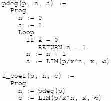
Fig. 1: Two fundamental routines used in the investigation
Using these ideas we are ready to state and develop the first of the results that are the subject of our discussion, The Division Algorithm. We use the following statement:
Let p(x) be a polynomial of degree n, and g(x) be a polynomial of degree m, with n>m, then there exist polynomials, q(x) and r(x), with the degree of r(x) < m such that
p(x) = g(x)×q(x) + r(x)
We verify the result by demonstrating the division process for finding q(x) and r(x) using long division for polynomials. While the CAS code for this process is straight forward, I strongly believe that every student needs to do this algorithm by hand after first learning about the algorithm. However, the process is a tedious procedure. If it is overdone, it gets in the way of what we want to accomplish in our course. What is a much better strategy is to have the students learn how one can teach it to the CAS. This is illustrated in Fig. 2
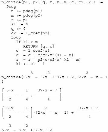
Fig. 2: The algorithm for polynomial division, its application and a check
Obviously, the students need to have had experience with the algorithm by having done some hand calculation, but once the process becomes mechanical for them, why not turn it over to the machine? The algorithm needs to be tested by the students. The last two segments of Figure 2 apply the algorithm to randomly generated polynomials and perform a check of the result. I have applied it to higher degree polynomials, but used third and second degree polynomials because of space considerations for the display in Figure 2. A polynomial of arbitrary degree and random integer coefficients (-a, a) can be generated with the Derive5 Command:
![]()
The students are now ready to reap the results of their work.
3 A student's excursion into pure mathematics - Elementary ideal theory
We now follow Böhm's agenda for exploring elementary number theory and apply it to polynomials. If our students are already familiar with the ideas of Greatest Common Divisor and Least Common Multiple for integers, so much the better.
We begin by applying the Euclidean Algorithm to two polynomials.
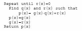
The students need to be convinced of three things. The first is that, because of the Division Algorithm, the loop condition will be met. The second is that the result does, indeed, divide p(x) and g(x), and the third is that it is the highest degree polynomial that can do so. The last two can be shown by a brief abstract discussion that traces the algorithm as follows:
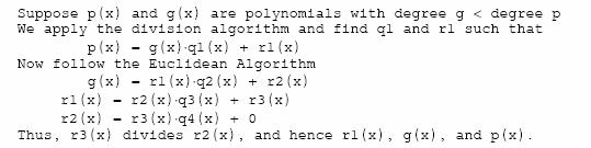
This argument certainly does not constitute a proof, but it contains the "idea of the proof" and has a sophistication that is at the level of secondary school students.
We can also use our previous work to trace the algorithm for specific cases. Since it is highly unlikely that two polynomials with randomly generated coefficients will have anything but a constant as a greatest common divisor, I generate examples by starting with a given polynomial and then multiplying it by first one random polynomial and then by another to obtain my two polynomials for an example.
After working with the Euclidean Algorithm, it makes sense to then use the CAS's built in factor function and arrive at an alternative method of finding the greatest common divisor (gcd) using the common factors. From this point on the discussion can proceed to the least common multiple and other topics of interest to the students and instructor. The fact is that the capabilities of the CAS allowed our students to explore some pure mathematics in a non-intimidating environment and with success. Furthermore, we did not use the CAS to produce "magic" results. It was a tool to extend the students abilities.
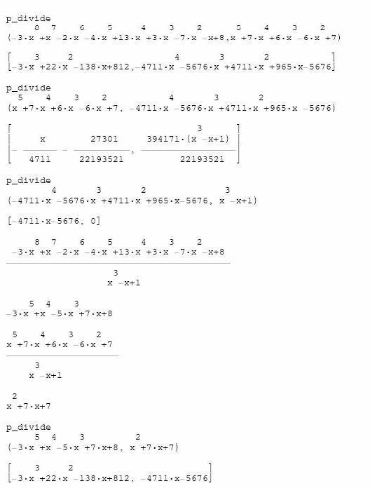
Fig. 3: Finding the greatest common divisor of two polynomials
4 The Remainder Theorem, polynomial expansion, and tangent lines
We begin with the Remainder Theorem, which is an immediate Corollary of The Division Algorithm.
Let p(x) be any polynomial of degree > 1, then if a is any real number, there exists a polynomial, q(x), of degree less than p(x) such that
p(x) = (x-a)×q(x) + f(a)
This result immediately establishes the connection between the real roots of a polynomial and its linear factors. We intend to use it in a different way. We will show how this theorem and our previous work with the CAS can lead to the expansion of any polynomial about x = a. From this expansion, we develop the idea of a linear approximation of a polynomial at that point.
Our basic result is that given a polynomial in the form
![]()
given any real number, s, we can find constants, a0, a1, …, an, such that
![]()
The "idea of proof " for the above result is a repeated application of the Factor Theorem.
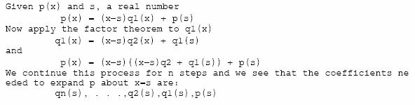
This process is usefully carried out by hand calculation for a first or second degree polynomials, but becomes tedious for higher degrees. It is easily mechanized with the CAS. Fig. 4 shows a Derive5 program and its application.
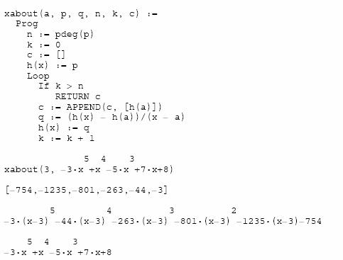
Fig. 4: Expanding a polynomial about x = 3
While the result is in itself interesting, students may have difficulty appreciating why such a process is at all useful. We need one more result that may be easily obtained. We state it in terms of percentages
If 1>x>0, then x2 is x×100% of x. Thus, if x is close to zero, it is significantly larger than its square and all higher powers of x.
This statement may seem awkward, but it justifies the next definition.
The linear approximation of a polynomial, p(x), about x = s is obtained from the degree 1 and degree 0 terms of the expansion of p(x) about x = s.
Note: I became aware of this method for finding the linear approximation of a polynomial about x=s from reviewing materials by Professor Warren Page.
We further enforce this definition by looking at the graphs of -3x5 + x4 – 5x3 +7x + 8 and -1235(x – 3) – 754, the last two terms in its expansion about x = 3.
|
|
|
|
|
Fig. 5: The graph of a polynomial and its linear approximation at x=3, y=-754 |
||
What a wonderful door has been opened for our students and us! It allows us to do many of the optimization applications from polynomial calculus. Furthermore, there is nothing artificial about our progression. It all follows logically from two of the most important theorems of the algebra our students are learning.
5 Application - Finding a smooth flight path
Consider the following problem posed as a situation from commercial aviation.
You are charged with programming an automatic pilot on a commercial airliner to find a smooth path from the aircraft's present height and distance to the runway where the plane will land. Suppose the airliner is at a height of h kilometers and a distance of d kilometers from the point on the runway where it will land.
If we make the assumptions that the runway is flat and that the airliner is flying at a level altitude, then we can assume that we need to find a curve with the following properties:
a) It passes through the point (-d, h).
b) It passes through the point (0, 0).
c) The line y=h is tangent to the curve at (-d, h).
d) The line y=0 is tangent to the curve at (0, 0).
We have four conditions on the curve. This means that we determine a polynomial with four coefficients, i.e. a cubic:
|
|
|
|
The first condition gives us the equation
|
|
|
|
The second yields
|
|
|
|
Thus, we need only find a, b, and g.
To use the third and fourth conditions, we use the fact that the tangent line to the curve at (-d, h) is y = h and at (0, 0) is y = 0. Both have 0 slope. Since the polynomial as given is the expansion about x = 0, we see that
|
|
|
|
We now examine the tangent line at (-d, h) using the program from the previous section. The resulting coefficient for (x + d) is d(3ad - b). The fourth equation is
|
|
|
|
Using the CAS to solve these nonlinear equations we have
|
|
|
|
Let's look at the resulting flight path when h = 1.5 and d = 6
|
|
|
|
|
|
Fig. 6: A flight path for 6 km away from the airport at a height 1.5 km |
|
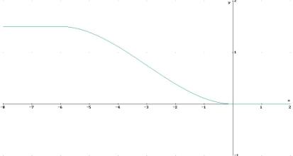
Reference
Böhm, J. (1998) "A Plea for Pure Mathematics". Keynote address presented at the Third International Derive/TI-92 Conference, Gettysburg, PA, USA.
Note: Copies of the Derive5 programs mentioned in this paper can be obtained from the author at the e-mail address given at the beginning of this paper. They will be sent by return e-mail as a Derive5 attachment.
Introducing Fourier Series with Derive
Alex J. Lobregt
Utrecht, The Netherlands
In electrical engineering courses functions such as the square wave Sq(t) and the saw tooth Saw(t), shown below, are frequently used.
|
|
|
|
Fig. 1: Square wave Sq(t) |
Fig. 2: Saw tooth Saw(t) |

These periodic functions of period
|
|
|
|
which satisfy certain conditions, may well be approximated by so-called Fourier Series.
|
|
|
|
The Fourier Coefficients an and bn are:
|
|
|
|
Example 1:
|
|
|
gives the graph: |
|
|
|
|
|
|
Fig. 3: Illustrating the sums of sine functions |
|
The Fourier Coefficients in example 1 are:
|
|
a n = 0 for n ³ 0 and |
|
for n ³ 1. |
The Utility file INT_APPS.MTH contains the function Fourier(f(t),t,a,b,n).
t is
the independent variable.
f(t)
is a periodic function.
[a,b]
is begin and end of one period.
n is
the number of the demanded harmonic terms.
Example 2
Find the first 5 harmonic terms of
|
|
|
|
|
File, Load, Utility INT_APPS.MTH
|
|
|
|
|
|
Fig. 4: Square wave |
|
Derive alllows to draw the single harmonic functions and their sum side by side, which gives an excellent insight into the structure of the Fourier Series |
(1) |
|
|
|
|
|
|
Fig. 5: Single functions to the left and the result of superimposition to the right |
|
After this introduction the underlying theory can be checked by calculating the following Fourier coefficients using Derive:
|
|
|
|
The result
|
|
|
|
can immediately be equated to the series in (1)
|
Exercise 1: Express the triangle wave using the standard CHI(a,t,b) function. (Use the Help function). Use Fourier(f(t),t,a,b,n) to find the first 6 harmonic functions. Plot the graph. Calculate the error at t = 1.5 |
|
|
Fig. 6: Triangle wave |
The use of complex numbers is especially important as it provides an opportunity for a theoretical review: The Fourier coefficients an and bn can be summarized as:
|
|
|
(2) |
The truncated Fourier Series then appears as
|
|
|
(3) |
Exercise 2: Use Derive to find the complex Fourier coefficients an of function f(t) from Exercise 1. Calculate separately the coefficient a0. Write the Fourier Series as shown in (3) for n = -3 ... 3 and Simplify. Check with the result of Exercise 1.
Help: As there will occur a problem for n = 0, split for n = -3 .. -1, n = 0 and n = 1 .. 3
Exercise 3: Take the square wave of example 2. Express the Fourier Series with respectively N = 10, 20 and 100. Plot all graphs into one screen. As you can see, the series comes closer and closer to Sq(t), however, the amount of overshoot nearby the discontinuities does not tend to zero with increasing N. Calculate this overshot with Derive. Compare your result with the limit
|
|
|
|
which amounts to 8.95% of the total jump. Until recently any investigation of this Gibbs Phenomenon used to be impossible, whereas in the present situation each student can perform calculations in this field.
Filtering
We can represent the amplitudes of the harmonic functions on a diagram, called the amplitude spectrum. The x-axis is labelled by the frequencies n w and the y-axis by |a(n)|.
Example 3: The square wave Sq(t) gives
|
|
|
|
|
|
|
|
|
|
|
(4) |
|
|
t |
|
|
|
Fig. 7a: Amplitude spectrum |
|
|
|
|
|
|
|
Fig. 7b: Harmonic functions |
|

Compare the amplitude spectrum with the separate harmonic functions in the plot of Fig. 7a-b
An application, which can be shown by means of Derive is a first step in the filtering theory. A low-pass filter is mathematically described by the convolution integral:
|
|
|
(5) |
with t being the bandwidth. In other words t is the maximum frequency, which slips by; see the amplitude spectrum in (4). If we now take
|
|
|
|
and t = 4 then, check the amplitude spectrum, only the 1st harmonic will be passed. We are not able to calculate (5) but plotting an approximation by means of Derive is possible.
|
|
|
|
|
|
|
|
|
|
Fig. 9: An approximation to the low-pass filter in (5) |
|
Exercise 4
Plot F(t) using integral (5) with t = 6 and check whether your expectation is confirmed.
Which value for t will pass by the 1st and 2nd harmonic?
Check your answer by plotting F(t).
The TI-89/92 as a tool for analytic geometry
Wolfgang Pröpper
Nürnberg, Germany
2. Points, lines and planes, their incidence and intersections
Calculators of the TI-89/92 series are computers with an integrated Computer-Algebra-System. And the emphasis is strictly on "Algebra", because typical algebraic problems, like solving equations, factoring expressions or plotting functions are handled by them flawlessly. The instructions required are in an easy way accessible through existing menus.
If however typical problems of Analytic Geometry are to be solved, and that is for instance entering a vectorial expression, solving a vectorial equation or projecting lines or planes from 3 to 2 dimensions, one is quickly faced with certain difficulties. To enter expressions one needs complicated manual operations and solving vectorial equations requires a complete rewriting of the system. Without a sound knowledge of the calculator's capacity, the user may have some difficulties in solving problems of that kind.
To overcome this problem, one can implement suitable procedures, which assist the user in Analytic Geometry. A second and much more important help is found in the custom menu facility of the TI-89/92. Using this technique the user has the opportunity to access an own menu, suitable for the problem, besides the standard menu of the home screen.
In this lecture a bundle of programs including a suitable custom menu are used and its possibilities are demonstrated. (The program group can be obtained from the author by sending him an email, referring to this paper.)
1 The geometry menu
|
In this case it is easily installed by calling menu_geo() from the home screen. Switching between custom and standard menu is simply achieved by [CUSTOM] ( = [2nd] [3]or [2nd] [HOME] at the TI-89). |
|
The items of the 6 new menus will be explained shortly as follows:
|
Muster[4] contains patterns for objects, which are typical for Analytic Geometry. One can see different vectors as columns and as rows, but also patterns of straight lines and planes in parameter form. They can easily be copied into the entry line and must then just be completed. |
|
|
Operat gives a direct access to important vector operations of the TI-89/92, which otherwise had to be typed in or had to be searched for in a relative awkward way in the [CATALOG]. |
|
|
Solve shows a choice of important operations for solving equations and systems of equations. They are standard with the TI-89/92 as well. But only item 2: solve can be found in the standard menu. |
|
|
Griech offers a quick access on Greek characters. |
|
|
Progs lists more custom procedures. Among them are vec2sys and vec2mat, which, as we will see, are very helpful in solving vectorial equations or trans and spieg, which do a good job at transformations of the plane. |
|
|
Tools contains instructions, which are also available in the standard menu for clearing home screen and so on. |
|
|
The program menu_geo is, as a glance into the program editor shows, a simple listing of the items (Item) in each menu, which are structured by corresponding titles (Title) and mounted by a Custom .. EndCustm construct. As far as that everybody can complete, extend and adjust this menu program to her or his special needs. |
|

2 Points, lines and planes, their incidence and intersections
The application of these menus and the functions included in them will now be illustrated with examples. First we turn towards classical analytic geometry in the R3 in which the relation of positions of points, straight lines and planes are investigated.
Points and straight lines
|
To enter a straight line, its pattern is copied into the entry line by [F1] [6]. Then you move the cursor to the left end of the line by [2nd] ßand type in the components, followed by a à. |
|
|
The term of the complete straight line is then stored as a function, for instance g1(l). The parameter l is obtained from [F4] [7]. In the same way (using [F1] [4]) the patterns of points are generated and then they are stored to p1 and p2. The vec2sys function (from [F5] [1]) in this case solves the vectorial equation p1=g1(t) and shows that P1 Î g1, but P2 is not lying on g1. |
|
(One can also see that the concept of vector functions for straight lines allows a very flexible handling of parameters. Instead of parameter l a parameter t or x or any other character can be used.)
Points and planes
|
Entering planes goes like in the previous example. The pattern of a plane is copied to the entry line by [F1] [7] and is filled with contents. Then the vectorial term is stored as a function of 2 variables, which must be called l and m in this case. |
|
|
Like before we ask the question if a point, (0|1|5) in this case, is lying in the plane. We first look at the corresponding equation and see a vector whose components are built up from a system of linear equations. |
|
vec2sys however does not solve the system in this case, but converts the vectorial equation. So one can make out a change in the order of the equations for instance, or, that the constant terms are collected on the right side.
By this the "secret" of the vec2sys function is revealed: The components of a column vector of Boolean expressions are transferred to a system connected with ands. And if the equations are sufficiently simple (for instance some of the equations hold only one variable) this leads to a solution of the vectorial equation in many cases.
|
In the problem at issue the system has still to be solved using the solve function (at TI-89/92Plus). The result shows, that the point lies on E1 (with parameters 1 and 2). |
|
Two straight lines
|
We add to the line g1, declared above, three more straight lines, called g2 to g4. With them we investigate the matters of intersection, parallelism and crooked location. |
|
|
The vec2sys function yields a definite solution in the case of g1 and g4 and shows that (-2|3|) is the intersection of both lines. With lines g1 and g2 or g3 respectively we just see that the system of equations is insoluble. Therefore this matter needs a further going investigation. |
|
|
For controlling we look at the vectorial equation g1(x)=g2(y). Another function, vec2mat, which is copied from [F5] [2] brings more clarity. She transforms the system of equations into a matrix. The columns are the coefficients of the system. The last column contains the constant elements, which are usually on the right side in an ordered system of equations. The other columns come according to the order of the solution variables as shown in the 2nd parameter of the function. |
|
A mathematician (hopefully!) sees already here, that the system of equations is contradictory. The function rref (from [F3] [1]) makes this contradiction clear in the 3rd line (0x + 0y = 1). As a consequence g1 and g2 are crooked.
|
Applying vec2mat to the equation g1(x)=g3(y) shows clearly that the directions of the lines are collinear. rref confirms this in the first two columns. The 2nd row however is contradictory, which shows, that g1 and g3 are really parallel. (In case g1 = g3 also the 2nd row would be a zero row.) |
|
Straight line and plane
|
To investigate the position of E1 and g4 the approach e1(x,y)=g4(z) is changed into a system using vec2sys, which is solved using solve. The result shows, that the plane is intersected by the line in (2|1|1). (For instance g4(0) or e1(3,2)). |
|
|
The vec<2mat function, in connection with rref solves this problem in just one approach. (And that can also be done with the original TI-92, which does not yet have the extended solve function.) |
|
|
In case of a straight line lying within the plane E1 there is no definite solution. However, taking the parameter of the straight line (i.e. z) as a free parameter, the parameters of the plane are depending from z in a simple form. |
|
|
If the straight line is really parallel to the plane, the solution with solve yields the result false, which means, the system of equations is unsolvable. (The solution using rref and vec2mat, which is not shown here, yields a contradictory 3rd row.) |
|
For the representation of planes there is another form instead of the parametric form: the so-called normalform. This normalform is very suitable for the investigation of the position of straight lines and planes or planes and planes. [5]
|
To show this, we store the vector of a point A1 and two directions v1 and v2 . The equation of a plane in normalform is first stored in a general way as a function nf with the three variables v ("coordinate vector"), n ("normalvector") and p (a point in the plane). The following call of the function nf yields the so-called normal or coordinate equation of a plane through A1 with directions v1 and v2 . |
|
|
Replacing the coordinate vector v in the attempt of a normal equation by the (vectorial) expression of a straight line (for instance by g1 or g4) one gets a simple equation for fixing the intersection point (or true or false). |
|
Two planes
|
Replacing the expression of a plane (for instance E1 with parameters l and m) instead of a straight line, we get a linear equation in just those parameters. Solving it for m and substituting the result in E1 we get the intersecting line s1 of the two planes. (Replacing s1 in the normalform yields true, what means that this line is also part of the 2nd plane. The vector expression of s1 is shown just for demonstration.) |
|
|
The "traditional" method using the functions solve ends at the same result. Substituting x=u+2 and y=u+1 into e1(x,y) yields an expression which differs from s1(l) at a first glance. |
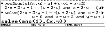
|
A simple comparison (using vec2sys again) shows that both straight lines are the same. |
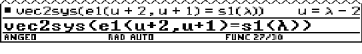
|
|
The method with the normal form yields true at equal planes, i.e. an identity. In case the planes are parallel however the answer is false, i.e. there is a contradiction. The reason is seen easily: The resulting equation has no more l and m, because the two directions and the normal vector are perpendicular. |
|
|
With equal planes vec2sys and solve lead to a correct result as well (however with clearly more expense). (In this case E2 was stored as a new plane and then compared with a plane through A1 with directions that are complanar to E2.) |
|
|
At parallel planes (the parallel now contains the origin) the solve function fails. She cannot yield a solution for the system of equations generated by vec2sys (claro!), but also she cannot identify it as contradictory (and yield false). But vec2mat in connection with rref shows the contradiction (in the 3rd line). |
|
Without much effort questions going beyond this, like problems of distance or the position of spheres relativ to the linear objects treated so far can as easily be answered.
3 Transformations
Another class of classical problems of analytic geometry in the R2 are transformations (or mappings).
From the different ways to show transformations from R 2 into R 2, we will treat those which have their numeric representation in the home screen and whose graphic results are visible in the graph screen. The procedures required for this are all found in menu [F5].
We always produce transformations of the triangle A(-4|-1), B(4|-3), C(3|2). The graph screen is set to ZoomDec as well as GRID and AXES in ON position.
|
The coordinates of the vertex points are assigned to variables a, b and c, using [F1] [2]. The function augm (from [F5] [3]) connects vector of the same rowdimension to a matrix. In this case the vectors a, b, c and a are written into a (2, 4)-matrix which is stored as d1. |
|
|
The function polygon (from [F5] [4]) does the plotting and connects the vertices in d1. (Because the triangle should be a closed figure, it is obvious, why point A occurs twice.) punkte (from [F5] [5]), with 1 as a 1st parameter marks the vertices with 3x3 pixel squares. (The names were added later, using the text tool [F7] [7]). |
|
Translation
|
Translating a point is simple. One has just to add the translation vector to the vector of the point in view. To translate a matrix like d1 however it makes sense to use a program. The function trans (from [F5] [6]) requires two parameters: the original vector and the translation vector. |
|
|
The coordinates of the transformed triangle can be seen in matrix d2. After the plotting is done one can see the original triangle and its transformation. The function punkte was, in this case, called with 2 as a 1st parameter in order to mark the vertices with small circles. (After returning to the home screen from the graph screen the standard menu turns up again. The geometry menu is reinstalled by pressing [CUSTOM] ( = [2nd] [3] or [2nd] [HOME] at the TI-89.) |
|
Dilation
|
For a dilation with factor k and center Z the following equation is valid:
To dilate triangle d1 from B with a factor 3/2 it has first to be translated by –b , then be dilated by 3/2 from the origin and finally be translated back by b again. |
|
|
For the plot the graph screen has to be cleared by ClrDraw ([F6] [4]) first, prior to plotting the triangle ABC (with squares as marks). Then the transformed triangle (with circles as marks) can be plotted. |
|
Rotation
|
A rotation of the R 2 with a rotation angle a around a center point D is done by
We first store the rotation matrix dr(a) and the vector d of the center. The transformation is again done in three steps: First we translate the triangle by -d, then we rotate it by 120° around the origin and finally translate it back by d. |
|
|
Plotting the original and the transformed triangle goes like in the previous example. The point of rotation is plotted with a 1st parameter 1 and a 2nd time with a 1st parameter 2. This leads to a third kind of marks: filled circles. |
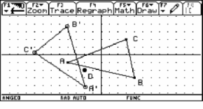
|
Reflection
The reflection of an object across a line g passing through a point P with direction v is described by
![]()
In that case n0 is the perpendicular unitvector of g, pointing to that half-plane which does not contain the origin. Because of the complexity of the transformation equation an extra program is useful to realize this transformation.
|
spieg (from [F5] [7]) needs 3 parameters: The 1st parameter is the original, the 2nd is a point on the reflection line and the 3rd is the direction of the reflection line. In this specific case the equation of the reflection line is stored as g(l) first. When calling spieg, g(0) gives a point on g and g(1)-g(0) gives the direction of that line. |
|
|
Drawing the triangle and its transformation goes like we did before. To draw the reflection line we use the procedure gerade (from [F5] [9]) which needs two points on the line (in this case g(0) and g(1)). |
|
Translation and reflection
|
As an example for linking transformations we look at a reflection of triangle ABC across AC and a translation by 2/3 CA. First we do the reflection after the translation and store the image as d2 for plotting. The reverse linkage, i.e. reflection first and then translation, shows that the result is independent from the order of each of these transformations. |
|
|
The instructions to generate the plot are the same as above and are not presented explicitly because of that. |
|
4 Projections
To display 3D objects in the plotting plane these objects have to be projected from R 3 on to R 2. In a first step we illustrate three common projections. Afterwards we apply this on the image of a tower.
Patterns of projections
To transform a point, which in this paper is handled as a 3D column vector, i.e. a (3, 1)-matrix, into a 2D column vector it must be multiplied from the left by a (2, 3)-matrix, the so called projection matrix.
Following we demonstrate for three projection matrices how a 3D cartesian coordinate system is projected. The columns of the projection matrix are the 2D images of the unit points on the (3D-) x-, y- and z-axis.
The program takes care of splitting the screen, installing the coordinate system and plotting the image, including marks of the unit points.
At Kavalierprojektion[6] the 3D y- and z-axes are mapped onto the x- and y-axes of the 2D coordinate system.
|
The projection matrix
is stored as kav. The 3D x-axis is rotated by an angle of 225°. By that, areas which are parallel to the plane of elevation are mapped undistorted. The image of the 3D x-axis predominates the projection. Using another angle yields another image. By using trig functions it is guaranteed that the units on all three axes remain units. |
|
The Militärprojektion keeps areas parallel to the ground plan undistorted. Therefore the image of 3D x- and y-axes are in a 90° angle. To emphasize the undistorted projection the (3D) z-axis is shortenend. If in addition the direction of the x-axis should be variable, we get an projection matrix depending on that angle:
|
It is stored as mil(a). The Figure to the right shows the coordinate system in that way, that the 3D x-axis is rotated by 210° against the x-axis of the 2D- coordinate system. |
|
At Isometrie the images of the 3D axes are all in a 120° angle.
|
To get the image of the z-axis looking upward, as usual the projectoin matrix iso takes the form (with angles in radians)
|
|
Projection of a tower
|
To demonstrate the projection of a 3D object a tower with a right-angled triangle base with the vertices A(1|4|-1), B(9|20|-1) and C(1|24|-1), a hight of 5 and the spire of the roof is at S(5|15|13) is generated. First the vectors of the base ABC and a hight vector h are entered. From that the upper base DEF can be determined. The following instruction stores the coordinates of the spire and then builds up, using the function augm, a (3D-) polygon p, that comprises all borderlines of the tower. p contains 14 points which means that each corner occurs twice. |
|
|
Now a matrix kav, that was generated previously, is assigned to a variable pro, which is used by the programs achsen and polygon. The origin of the coordinate system is translated from the center of the screen by 5 units to the left. To construct the tower we now just have to call the procedure polygon with a parameter p. The names of the corners and the axes as well as the text were added afterwards, using the text tool [F7] [7]. Of course it would be possible to add more points, like units on the axes or intersection points of the edges with the x-y-plane. The function punkte, which can also be called with single points as parameters would alow that. |
|
|
|
|
|
Both images to the right show the same tower, once in military projection, the other time in isometric projection. The axes are named in each case and the parameters of the mapping are specified. |
|
|
|
|
References
Geyer, H. R. (1999) Platonian Solids – Hidden Lines with TI-92. Derive News Letter # 35.
TI-92 (1995) Guidebook. Texas Instruments.
TI-92 (1998) Das TI-92 Plus-Modul, Ergänzung zum TI-92 Handbuch. Texas Instruments.
TI-89 (1998) Handbuch. Texas Instruments.
Weller, H. (1997) Darstellung von Polyedern – Platonische und archimedische Körper im Mittelpunkt. Derive News Letter # 27.
Weller, H. (2000), Darstellung von Objekten mit dem TI-92. TI-Nachrichten, Ausgabe 1/2000.
The use of CAS in the Thuringian school system: Present and future
Karsten Schmidt
Schmalkalden, Germany
In this paper we present results of a survey, carried out in spring 2001, of all 336 secondary modern, 106 grammar and 5 comprehensive schools of Thuringia, one of the 16 states of the Federal Republic of Germany. 234 (52%) of the 447 schools filled out and returned the questionnaire; the response rate was the highest from grammar schools, the lowest from comprehensive schools. The questionnaire was to be filled out by the head math teacher, alternatively by another math teacher.
The survey was preceded by a pilot study of all 26 secondary modern and 8 grammar schools in 2 Thuringian counties (response rate 94%; carried out as interviews). Besides the aim of gaining experience with a first version of the questionnaire, it also was carried out to obtain typical answers to the two open questions on advantages and disadvantages of the use of symbolic pocket calculators (PoCs) or computer algebra systems (CAS) in math lessons.
Based on the respective median or mode, an average school has one PC lab with 11 workstations in a Windows NT network. The workstations have a Pentium II processor with 300 MHz, 63 MB RAM and a 3.65 GB hard disk, running under Windows 98.
|
There is apparently some uncertainty in the schools about the availability of PCs in pupils’ homes. The request “Please estimate the percentage of 10th grade pupils having access to a PC at home” yielded answers between 10 and 99%. The distribution of these answers can be found in the histogram in Fig. 1; the median is 60%. |
|
|
Fig.1: PC at home (10th grade) [%] |
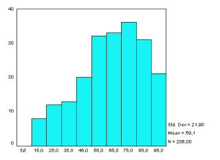
The question regarding the grade in which graphical or symbolic PoCs are first used in math lessons gave the result to be expected for this state, namely that graphical PoCs are not used at all and symbolic PoCs are used only at some schools taking part in a project of school development.
It was then asked in which grade the teacher filling out the questionnaire would like to start using graphical (symbolic) PoCs in math lessons. Of the 133 (118) schools that replied to this question 60 (76) chose "not at all"; the other 73 (42) schools would like to use graphical (symbolic) PoCs in math lessons. If we only consider those who answered this question, then 55% (36%) would like to use graphical (symbolic) PoCs. If we add all schools that didn’t answer this question at all to the group of schools that replied "not at all", the percentage would drop to 31 (18).
The mode shows that a relative majority of the schools that would like to use graphical (symbolic) PoCs would like to do so as of the 10th (11th) grade. The mean value is 9.9 (10.2).
|
“How well do you know the following symbolic PoCs and CAS?” For this question the following answers were possible: o never heard of it o heard of it o basic knowledge o good knowledge If we code these by 0 / 1 / 2 / 3 (and count no answer at all to the answer possibility “never heard of it”), the mean values represented in Fig. 2 demonstrate that the teachers who filled out the questionnaire have a relatively weak knowledge in this field. |
|
|
Fig. 2: Knowledge of various CAS |
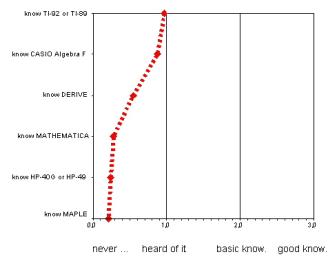
The answers to the question “How often do you personally use symbolic PoCs or CAS?” are no surprise in the light of the previous result. If we code the 4 answer possibilities “never” / “rarely” / “frequently” / “very often” 0 / 1 / 2 / 3 (and count no answer at all to the answer possibility “never”), we get as mean values 0.54 and 0.55, respectively. Symbolic PoCs (CAS) are used “very often” or “frequently” by only 13% (14%) of the teachers asked.
The final question was
“Which THREE of the following statements about symbolic PoCs and CAS are, in your opinion, the MOST correct?”.
The answer possibilities were:
|
|
|
|
|
As mentioned earlier, these predefined answer possibilities were simply the 6 most frequently given answers to the two open questions in the pilot study on advantages and disadvantages of the use of symbolic PoCs and CAS in math lessons. This practice may have resulted in a bias towards the disadvantages since these seem rather complete while, for example, the obvious advantage, that by using symbolic PoCs or CAS teachers gain more time for working on interesting and more realistic problems, is not included. The relative frequencies of the answers given can be found in Fig. 3. |
|
|||
|
Fig.3: Advantages and disadvantages of PoCs and CAS |
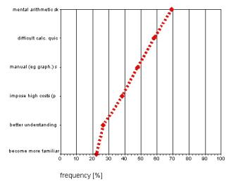
Most frequently marked (by 69% of the questioned teachers) was one disadvantage, namely that mental arithmetic skills weaken. The second most frequently marked answer possibility was one advantage: 58% think that difficult calculations can be done quickly and correctly with technology. The two other disadvantages (weakening of manual skills: 48%; high costs: 38%) and finally the two remaining advantages (better PC understanding: 26%; increased familiarity with PC: 22%) follow.
195 (83%) of the teachers who filled out the questionnaire stuck to the rule to mark exactly 3 answer possibilities out of 6. If we deduct the 11% who didn’t answer this question at all, only 6% marked more, or less than 3 answer possibilities.
Requiring the respondents to mark exactly 3 statements out of 3 advantages and 3 disadvantages resulted in a decision pro or contra the use of symbolic PoCs and CAS in math lessons: the teachers who filled out the questionnaire had to decide on there being either more advantages or more disadvantages. Within the 195 schools that stuck to the rule the following picture arose: 13% marked only disadvantages, 51% marked 2 disadvantages and 1 advantage, 34% marked 2 advantages and 1 disadvantage and 2% marked only advantages. In total, 64% see more disadvantages and 36% more advantages from the use of symbolic PoCs and CAS in math lessons.
Examining only the (59) grammar schools in the data set we find some interesting deviations from what we found for all schools together.
The teachers who filled out the questionnaire estimated that the portion of the pupils in the 10th grade who have the use of a PC at home is between 20 and 96%, the median is 77.5%. A majority of the grammar schools has at least 2 PC labs. 46% of the grammar schools have a license for a CAS (compared to only 4% of all secondary modern schools).
Asking in which grade the teacher filling out the questionnaire would like to start using graphical (symbolic) PoCs in math lessons, we got the following results: of the 44 (40) grammar schools that replied to this question 7 (10) chose "not at all"; the other 37 (30) schools would like to use graphical (symbolic) PoCs in math lessons. If we consider only those who answered this question, then 84% (75%) would like to use graphical (symbolic) PoCs. If we add all the schools that didn’t answer this question at all to the group of schools that answered "not at all", the percentage would drop to 63 (51).
|
The mode shows that a relative majority of the grammar schools that would like to use graphical (symbolic) PoCs would like to do so as of the 11th (10th) grade (mean values 10.1). The question “How well do you know the following symbolic PoCs and CAS?” (no answer or “never heard of it” = 0 / “heard of it” = 1 / “basic knowledge” = 2 / “good knowledge” = 3) partly revealed noticeably better knowledge of the questioned teachers in grammar schools. The 6 corresponding mean values are represented in Fig. 4. |
|
|||
|
Fig. 4: Knowledge of CAS in grammar schools |
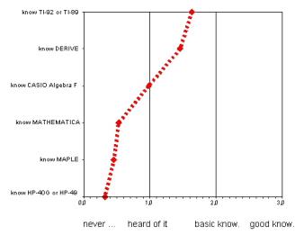
Accordingly, the question “How often do you personally use symbolic PoCs or CAS?” (no answer or “never” = 0 / “rarely” = 1 / “frequently” = 2 / “very often” = 3) gave as mean values 1.05 and 1.25, respectively. Symbolic PoCs (CAS) are used “very often” or “frequently” by 31% (36%) of the teachers at grammar schools.
To the final question, about the 3 most important advantages and/or disadvantages of the use of symbolic PoCs and CAS, the most frequently selected statement (80%) at grammar schools was an advantage, namely that difficult calculations can be done quickly and correctly with technology. This is a deviation from the value of all schools together by 22 percentage points. The second largest deviation also arose in the context of an advantage (better PC understanding: 34% compared to 26%). The other deviations were between 2 and 4 percentage points.
Within the 56 grammar schools (95%) that marked exactly 3 answer possibilities the following picture arose: 9% marked only disadvantages, 50% marked 2 disadvantages and 1 advantage, 37% marked 2 advantages and 1 disadvantage and 4% marked only advantages. In total, 59% see more disadvantages and 41% more advantages from the use of symbolic PoCs and CAS in the math lessons.
Computers and Computer Algebra Systems
in engineering education
Rolf Wasén
Norrköping, Sweden
1 Introduction
There are in fact several aspects on using computers in engineering education. One is the rather obvious that the students shall learn to use computers in their future mission as engineers, for calculations as well as for design and exploration of ideas. The other is the less obvious use of computers for improving learning and understanding. That is, we have the aspects of computers as a tool in engineering work and the computer as a learning tool. In this article we will mainly focus on the latter aspect. There are a number of subjects to which the computer may be applied but here we will focus on the conceptual aspects (see Wasén 1996). Wasén (1988) and Forster (1989) give an outline of the new possibilities in chemistry. Since mathematics is the formal part of the language of science going like a red thread through science and its applications we will mainly focus on the use of computers for understanding and performing mathematical computations. Here too we have a distinction between software for numerical or more symbolic mathematics. But since distinctions always are diffuse and since we want to stress the links between different areas we will not solely focus our attention on just one topic. Instead we try to imagine the engineering profession as a whole. A successful implementation of computers may demand a synthetic approach to engineering education.
Problems
There are a number of objections to the use of computers in the basic mathematics courses. The main one is that the traditional skill required for the handling of mathematics will dwindle with the use of computers for manipulations that now are done by hand. To some extent this have happened with the use of pocket calculators in high school. To counterbalance this I think that there is a need of stressing the concepts and understanding of mathematics. Besides this the students should learn how to structure expressions and calculations before they proceed to the computer. Irrespectively how the calculations are performed they have to be able to judge their soundness and correctness! It would also be of great help if the software systems, and in particular the CA-systems would provide with a step-by-step mode for the more basic operations. Another basic problem is the overhead that the computer and software generates. Still the greatest obstacle for the use of computers in education is the very fact that they are too bulky, noisy and expensive! On the top of this we have the problem with costs for purchasing and handling the necessary software. The material problem technology will solve for us if we demand it and the prices for CA-software has already dropped to reasonable levels. So we may proceed towards solutions of the other problems.
A model for the use of CA-Systems in math education
A minimal requirement is that the students understand the core of the theory and be able to manually perform at least three simple calculations by hand. The students that want to proceed by more calculations by hand should be allowed to do so. The time saved could be invested in more thorough explanations of the basic concepts and in learning the skill to structure expressions (and calculations). For the high school level Sjöstrand and Wasén (1992) have developed some kind of model for the introduction of CA-systems.
Particularly tedious and error-prone is the partial fraction decomposition. It can now be swiftly done by means of CAS like Derive, Maple, or Mathematica. Instead we should now try to explain Euclid’s algorithm carefully since it is instrumental for the construction of efficient basic algorithms. Also more time should be devoted to explaining how calculations with symbolic or parametric expressions work since this is at the core of the use of CA-systems. In fact, this is quite carefully done at the basic math courses at ITN.
Then there is a need of better exploiting the common threads between the different disciplines of engineering education. This will save time. Part of this time should be re-invested in giving the students more time for reflexion and also for working with a basic course in a leisurely pace. This basic course should contain the essentials of discrete mathematics and the historic background including the notions of machine, algorithm and computer programs. Rightly communicated such a course could be a source of inspiration as well.
Project works
At ITN the students in the basic courses in calculus are assigned project works. This I took as an opportunity to introduce computers and computer programs into their world of mathematics and mathematical modelling. However, a requirement was that this should come in naturally and, in fact, there were a couple of groups that did not use computers at all (but for plotting solutions). The tasks were the following:
(1) General characteristics of a CA-system like Derive
(2) The magic of complex numbers
(3) Code for first-order linear differential equations with general coefficients
(4) Code for second-order linear differential equations
(5) Laplace transforms with the support of CA-systems
(6) Modelling of a couple of types of chemical reactions
(7) Modelling of the spring without damping
(8) Modelling of time evolution of concentrations in communicating containers
(9) Exploration of the relation between roots of equations and fixed-points of functions
The students were divided into groups consisting of 4-5 people. They were assigned the tasks and expected to work 10 hours with them ending-up with a written report and an oral presentation in front of the class. The students that used computers were specially instructed to deal with the correctness issue.
2 Our approach
Experiences from project works
In general the students found it fun and rewarding to work with the computers for mathematical problem solving. This in particular with an easy-to-use CA-system like Derive. As one student expressed it ”Derive is quite intuitive. Mostly it does what you expect it to do.” Since they previously had done everything by hand they had no difficulties in seeing the extraordinary power that the computer support may give them. Occasionally they also saw the limitations. There was a large span in skills in dealing with the programs.
The group assigned the task (1) clearly sensed the difference
between symbolic and numeric computing and so also between symbolic programs
(CAS) and more numerically oriented programs like MATLAB. This distinction is
not always sensed among industry or research people. One group member explained
the capabilities of Derive to his fellow classmates in the following way: ”It
does what we are sitting and doing by hand all the time”(!).
As to (2) one student told me: ”During the same day I saw the
appearance of complex numbers in different forms in three different subjects”
(!!). Actually, one student – in order to graphically illustrate that complex
numbers may stand for rotations – cleverly used the capabilities of Derive
generating his own ”code”. The net result was that he made a hand of cards out
of one card iteratively rotated by a certain amount (around 18 degrees).
When working with (3) the groups quickly saw the limitations with
CA-computing. They were a little disappointed but also content with being able
to construct the code from basic principles (that they understood and could
explain to the class).
With (5) the students showed great ingenuity in fiddling around with
the inverse transformations.
Finals, the group working with (8) first made a little ”theory” for
the connection between fixed-points and roots and as they expressed it –
strengthened by this understanding – went on to illustrate different cases
including chaos (sensitive dependence on initial conditions) graphically in
MATLAB.
Extensions of project works into research projects
There are a number of attractive possibilities to extend project works with elements of computer programming into research projects. Three examples will illustrate the possibilities:
Simulation of non-linear dynamical systems
In project work (9) the students were in fact working with one aspect of non-linear dynamical systems. Namely the simulation of a simple but archetypical equation – the logistic equation – as well as some other equations. That is, discretised and non-linear dynamic systems. This subject is very apt for computer processing. Interestingly enough the modern branch of the theory of dynamical systems started with post-war experiments with computer simulations of non-linear equations (representing coupled oscillators) See for example “Studies of Non Linear Problems” (Fermi-Pasta-Ulam) in Ulam (1990). There is an attracting possibility to extend the more conventional course material on linear oscillators into material on damped and driven oscillators coupled linearly or non-linearly. This subject boards naturally with bioscience.
See http://www.itn.liu.se/~rolwa/Nonlinear_course.html.
Rational approximants and signal processing
Rational or Padé-approximants (sometimes called Padé-Hermite approximants) of functions of one variable are generalisations of the ordinary Taylor series that in many respects are superior. They model poles of finite order much better and their range is often also far better. But they are not very well suited for hand calculations! Some historic background will not hurt. For example, why are these rational approximants called Padé or Padé-Hermite approximants? Freeman (2000) made some interesting use of them in neurodynamics.
Discrete version of the concept of radius of curvature
In our analysis courses the students learn to analyse smooth curves in space and so how to compute their radius of curvature, torsion et cetera. But in the measurement-based life we experience the raw data is often time-series or arrays of points and so necessarily of a discrete kind. But there is a discrete counterpart to the concept of radius of curvature for polygonal chains that is used in bioinformatics (reference to Soumpasis). This subject has a natural connection with Euclidean plane geometry. The resulting formulas are complicated even if the principles are simple and well known from their courses in linear algebra (provided that they know their Euclid!) and analysis. These kinds of ideas can be used in more elementary classroom contexts as well. For example, we may imagine a car following a curve of a certain kind (“dog turn” for example); illuminate it with stroboscopic flashes; measure and calculate its position by means of two direction measurements; and finally plot the radius of curvature along the path with histograms or colour coding.
A mathematics study centre (”Mattetek”)
At the Institute of Science and Technology at Norrköping we have a little Mathematics Study Centre, where the students get teacher assistance from experienced mathematicians and teachers and occasionally older students. It consists of a room, two computers with the appropriate software and a small collection of books and other helpful material.
Here the students work with their exercises, discuss mathematics and occasionally use the computers for mathematical calculations. Their main issue is the understanding of basic mathematics including logic, algebra and how to structure and solve mathematical problems. For this human communication, teaching, discussions and reflection are needed but computer algebra programs like Derive has turned out to be a very valuable tool for illustrating ideas and checking results. This not at least for the teacher (!). It is also a fine tool for the establishing of reliable solutions (software form of Solution manual).
Since the students have to acquire the capacity to solve mathematical problems by hand and do need to train this in the first hand. But close to examinations there may not be time to go through all calculations. Then a tool like Ca-systems (CAS) is useful since it permits the accurate and swift verification of the ”Ansatz” to the problem. One student using Derive on a hand-held computer claimed that this was a very appropriate tool that had helped him to get the highest grade in mathematics.
3 Summary remarks
Judging from my experiences from high-school education to research and industrial applications I think that the proposed model for the use of CA-systems and other kinds of more sophisticated software only can be provisory. A lot of work is needed in order to get all the pieces on place and the question is also how to get all this into a working classroom education. Certainly some deeper thoughts about the goals with university teaching, and the subsequent necessary differentiation of the teaching, are needed. The students already have to learn more than they can manage both in terms of time and complexity. So above all is needed a basic course focused on understanding and reflection and less on computing and proving. This basic course should give a common theoretical basis for all of the engineering courses and so have to contain elements of discrete mathematics and how these elements are used in the different applications. Moreover it has to contain the basics of how to formalise facts in terms of symbolic relationships and how this is used in the programming languages. This basic course should run for a year and could be ended with an optional summer school. In this summer school a simple introduction to current research should be given and project works boarding to research distributed and discussed. Certainly, with such a basis, much more could be adsorbed during the second and third year!
Acknowledgement. I am indebted to colleagues at ITN and students from NM2C and NO2B for interesting suggestions and comments.
References
Wasén, R. (1996) Conceptual Engineering: Where Theory and Practice Meet. Alan, E.A. and Steiner, J.M. (eds.) The Role of Mathematics in Modern Engineering. Proc. of AEMC 94. Studentlitteratur, Lund.
Wasén, R. Computer Algebra - Software for symbolic mathematics - Also a possibility for chemistry?
Gasteiger, J. (1988) Software Entwicklung in der Chemie 2. Springer.
Sjöstrand, D., Wasén, R. (1992) Experiments with mathematics - Derive in the teaching. Onsala (in Swedish).
Forster, P., Khuen, A., Wasén, R., and Ziessow, A. (1989) Computer Algebra in chemistry. Computer Application in the Chemical Industry. VCH Gesellschaft, Weinheim, 613-622.
Ulam, S. M.(1990) Analogies between analogies. Bednarek, A. R. and Ulam, F. The Mathematical Reports of S. M. Ulam and His Los Alamos Collaborators. Univ. California Press, Berkeley.
Freeman, W. J. (2000) Neurodynamics; An Exploration of Mesoscopic Brain Dynamics. Springer, London.
Soumpasis, D. M. Paper outlining an Erlangen Program for Mathematical Bioinformatics.
Loci - Ortskurven
Wilhelm Weiskirch
Stadthagen, Germany
Short English version of the paper
1. Loci of special points of the triangle
4. Mirror images of elementary curves
Curves are a lot more than function graphs. In teaching mathematics mostly the concept of a curve is reduced to the graph of a function. Doubtless this treatment of the "curve" does not nearly exhaust its mathematical meaning and its didactical possibilities. Especially geometrical approaches to nontrivial curves and their analytical inspection are now possible by means of Dynamical Geometry Systems and Computer Algebra Systems as well. Doing so we could contribute in breaking the recent inflexibility of mathematics teaching in secondary school level 2. Applying the genetic method we will discuss nontrivial curves generated as loci of dependent points and their importance and chances for math education. Some examples are given in this paper. The full paper can be found in the extended version in German.
1 Loci of special points of the triangle
Example: Inspect the locus of S with C moving on a circle around A.
|
|
|
|
|
Fig. 1: To find the locus of S while C is moving on a circle around the centre A |
||

2 The conchoid
See some TI-92 screen shots of four varieties:
|
|
|
|
Fig. 2 a, b: Types of conchoids |
|
|
|
|
|
Fig. 2 c, d: Further types of conchoids |
|

3 Trochoids
The cycloid
|
|
|
|
|
|
Fig. 3: Movement leading to the cycloid |
|
|
|
|
|
|
Depending on h, we obtain three forms of the cycloid:
|
|
|
|
|
|
Fig. 4: Types of cycloids |
|
|
h < r |
h = r |
h > r |

Using a DGS like Cabri the students can generate their own models and study the various forms of curves:
|
|
|
|
|
Fig. 5: Generating a cylcoid by a DGS |
||
How to generate epitrochoids and hypotrochoids
|
|
|
|
Fig. 6a: Epitrochoid: K1 rolls outside of K0 |
Fig. 6b: Hypotrochoid: K1 rolls inside of K0 |
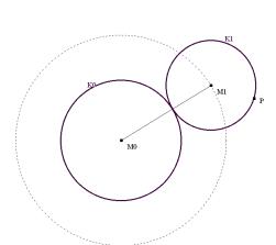
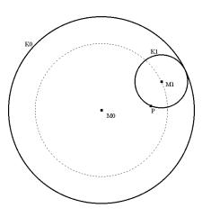
Some trochoids
|
|
|
|
Fig. 7a-c: Some trochoids |
|


|
|
|
|
|
|
|
Fig. 7 d–g: Further trochoids |
|


4 Mirror images of elementary curves
|
Find an analytical way to obtain the mirror image of the standard parabola with respect to the straight line y = 2x – 3. Other questions are like What is the resulting curve mirroring the x-axis with respect to the parabola? |
|
|
|
Fig. 8: Mirror image of a parabola |
References
Fladt K. (1962) Analytische Geometrie spezieller Kurven. Akademische Verlagsges., Fankfurt.
Gray A. (1994) Differentialgeometrie. Spektrum Akademischer Verlag, Heidelberg.
Kreul and Kreul (1989) Funktionen und Kurven Bd. 2. Verlag Harri Deutsch, Leipzig.
Kreyszig E. (1957) Differentialgeometrie. Akad. Verlagsgesellschaft Geest & Portig, Leipzig.
Kroll and Vaupel (1986) Analysis für den Leistungskurs Bd. 2. Dümmler, Bonn.
Kühnel W. (1999) Differentialgeometrie. Vieweg, Braunschweig/Wiesbaden.
Lehmann E. (1990) Lineare Algebra mit Vektoren und Matrizen. Metzler Verlag.
Meyer J. (1996) Kegelschnitte mit Geometrie – Software.Mathematik betrifft uns Nr.5.
Meyer J. (1998) Von der Normalparabel zu kubischen Kurven. Beiträge zum Mathematikunterricht. Franzbecker, Hildesheim.
Steinberg G. (1998) Evoluten und Evolventen. MU Heft 4-5.
Steinberg G. and Ebenhöh, M. (1998) Ausgewählte Aufgaben zur Analysis. Schroedel, Hannover.
Strubecker, K. (1964) Differentialgeometrie I / II / III. Sammlung Göschen, Berlin.
Wieleitner H. (1908) Spezielle ebene Kurven. Göschen Verlagsbuchhandlung, Leipzig.
Wünsch, V. (1997) Differentialgeometrie. Teubner Verlag, Stuttgart.
Loci - Ortskurven
Wilhelm Weiskirch
Stadthagen, Germany
Extended German version
2. Ortslinien besonderer Punkte im Dreieck
Kurven sind mehr als Graphen von Funktionen hat Günther Steinberg seinen Aufsatz in der MU 1996 betitelt. Dies ist in der Tat aus zweierlei Gründen richtig
Historisch
gesehen befasst sich die Mathematik seit mehr als 2 1/2 Jahrtausenden mit Kurven und noch kein
1/2 Jahrtausend mit Funktionsgraphen.
Funktionsgraphen
sind lediglich Visualisierungen arithmetisch - algebraischer Zusammenhänge und
zwar nachträgliche, während Kurven verschiedenster Art um uns herum präsent
sind in Natur, Kunst und Technik und erst nachträglich analysiert werden.
1 Einleitung
Kurven sind
Darstellungen
der Bewegungslinien von Körpern
Linien,
die sich bei der Durchdringung von Körpern zeigen
Hilfen
für die Beschreibung von Formen
Ortslinien
einer Menge von Punkten gleicher Eigenschaft
Graphen
von Funktionen
Die weitverbreitete Reduktion des Kurvenbegriffs auf das Bild einer Funktion in unserem derzeitigen Mathematikunterricht führt dazu, dass dessen mathematische Bedeutung und das hohe didaktische Potential nicht annähernd ausgeschöpft wird.
Die Bedeutung des Kurvenbegriffes für einen problem- und anwendungsorientierten Mathematikunterricht ist zum einen in der Rolle des zentralen Mathematisierungsmusters und zum anderen darin zu sehen, dass sich Kurven in vielfältiger Weise realisieren und variieren lassen und somit für Schüler zu überraschenden und interessanten Entdeckungen führen.
durch
Apparaturen oder Materialien( Spirograph zur Konstruktion von Rollkurven)
durch
Fadenkonstruktionen
durch
Schnitte von Flächen und Körpern
durch
Konstruktion von Krümmungskreismittelpunkten
durch
Graphikprogramme
durch
dynamische Geometriesoftware
Spielten die Kegelschnitte schon seit Jahrzehnten in der Schule und in der didaktischen Diskussion eine wichtige Rolle – mal abgelehnt , mal intensiviert befürwortet – so ist in der heutigen Diskussion zunehmend die Vielfalt von Kurvenphänomenen zum zentralen Gegenstand geworden.
Entscheidende Aspekte für eine Realisierung im Unterricht könnten sein
Art
und Zugang von Realisierungen und von Experimentiermöglichkeiten
Relevanz
und Vielfalt der Hypothesen, die sich aus den Experimenten ergeben
Zusammenhänge
zu anderen Inhalten des Mathematikunterrichts
Anwendungsrelevanz
Bei eingehender Betrachtung des Themenkreises Kurven offenbart sich schnell eine Fülle von Phänomenen und der Reichtum an Bezügen und Vernetzungen. Unterricht wird geprägt durch eine reiche Beziehungshaltigkeit von Analysis, analytischer Geometrie und linearer Algebra.
2 Ortslinien besonderer Punkte im Dreieck
Am Beispiel der Schnittpunkte von Transversalen im Dreieck soll gezeigt werden, dass schon in der Sek I (bei uns Klasse 7 bis 10) unter Benutzung einfacher dynamischer Geometriesoftware nicht triviale Kurven erzeugt werden können und von ihrer Genese her erste Untersuchungen nahe legen.
|
I |
Betrachten Sie die Ortslinie des Schwerpunktes, wenn sich der Punkt C auf einer Parallelen zu AB bewegt. |
|
|
|
|
Fig. 1 |
|
II |
Betrachten Sie die Ortslinie des Schwerpunktes, wenn sich ein Punkt des Dreiecks auf dem Umkreis bewegt. |
|
|
|
|
Fig. 2 |
|
III |
Betrachten Sie die Ortslinie des Schnittpunktes S, wenn sich C auf einer Parallelen zu AB bewegt |
|
|
|
|
Fig. 3 |
|
IV |
Betrachten Sie die Ortslinie des Schnittpunktes S, wenn sich C auf dem Kreis um A bewegt |
|
|
|
|
Fig. 4 |
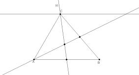
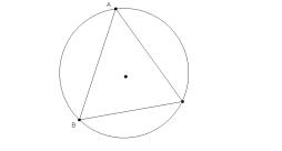
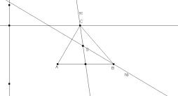
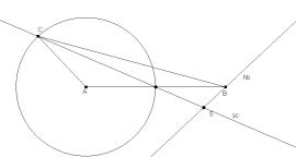
3 Rund um die Konchoide
Gegeben ist eine feste Gerade g . Ein Strahl h dreht sich um einen festen Punkt Z. Vom Schnittpunkt Q des Strahls h mit der Geraden g wird nach beiden Seiten die gleiche Strecke der Länge a abgetragen.
Die so gefundenen Punkte P1 und P2 liegen auf einer Kurve, der Konchoide (Muschellinie).
Beispiel 1:
g ist parallel zur x-Achse im Abstand b = 3, der Drehpunkt ist der Ursprung.
Mit Q(t|b) gilt für die Ortsvektoren von P1 und P2 :
|
|
|
und |
|
|
Für den normierten Richtungsvektor des Strahls gilt dann
|
|
|
|

und somit insgesamt
|
|
|
|
|
Die Konchoide hat dann die Darstellung
|
|
|
, tÎ3 |
|
|
Für b = 3 und die Streckenlängen a = 2;3;4 ergeben sich die Kurven: |
|
|
|
Fig. 5 |
Beispiel 2:
g ist eine Ursprungsgerade mit der Steigung 1; der Drehpunkt ist S(3|1).
Für Q(t|t) erhält man auf ähnlichem Wege wie oben
|
|
|
|
|
und damit die Parameterdarstellung der Konchoide
|
|
|
, tÎ3 |
|
|
Für die Streckenlängen a = 1 und a = 3 ergeben sich folgende Graphen: |
|
|
|
Fig. 6 |
Beispiel 3:
Die Strecken a werden jetzt vom Schnittpunkt Q der Strahlen mit der Normalparabel abgetragen.
Für S(0|4) und Q(t|t2) erhält man wie oben die Parameterdarstellung der zugehörigen Konchoide
|
|
|
, tÎ3 |
|
|
|
|
|
|
|
Fig. 7: Konchoiden für a=1 und a=2 |
|
Fazit:
Allgemein ergibt sich analog für eine Funktion f und einen festen Punkt S(c|d) die Konchoidendarstellung
|
|
|
, tÎ3 |
|
Beispiel 4:
|
Dreht man einen Strahl um einen Punkt A und trägt man jeweils von seinem Schnittpunkt mit einem Kreis durch A mit dem Radius r eine Strecke gleicher Länge a nach beiden Seiten ab, so erhält man die Punktmengen Pi und Qi. Bestimme die Ortskurve dieser Punktmengen. Für a=2r ergibt sich die so genannte Herzkurve oder auch Kardioide. |
|
|
Fig. 8: Kreis K mit M(4/0) und r = 4 und Pascalsche Schnecke für a = 2 |
4 Rollkurven
Die Übertragung einer Drehbewegung durch Zahnräder soll gleichförmig, d.h. ruckfrei und kontinuierlich sowie reibungslos sein. In der Feinwerktechnik – z.B. bei mechanischen Uhren - verwendet man als Zahnflankenform die Zykloidenform. Zahnräder mit einer solchen Zykloidenverzahnung weisen ein sehr gutes Abrollverhalten auf und unterliegen deshalb einem sehr geringen Verschleiß auf den Zahnflanken.
Eine Zykloide entsteht, wenn man die Ortskurve eines Punktes einer auf einer Geraden rollenden Scheibe betrachtet.
|
|
|
|
Aus der Abhängigkeit von dem Roll- oder Wälzwinkel j bzw. t (im Bogenmaß ) ergibt sich die Parameterdarstellung:
|
|
|
|
|
Liegt der fest mit der Scheibe verbundene Punkt P nicht auf dem Rand, sondern in einem Abstand h zum Mittelpunkt, dann erhält man eine leicht geänderte Darstellung:
|
|
|
|
|
In Abhängigkeit von h ergeben sich die folgenden drei Typen:
|
|
|
|
|
|
Fig. 10: Typen von Zykloiden |
|
|
h < r |
h = r |
h > r |

Diese Abhängigkeit lässt sich graphisch auch sehr eindrucksvoll mit dynamischer Geometriesoftware wie Cabri oder auch Euklid experimentell erschließen. Über diese Visualisierung eines durchschaubaren geometrischen Zusammenhangs sind die Schülerinnen und Schüler motiviert, anschließend diese Kurven auch algebraisch zu beschreiben und dann zu erzeugen. Zwei dieser Möglichkeiten sind in folgenden Bildern dargestellt.
Beispiel für die DGS Euklid
|
|
|
|
|
|
Fig. 11 |
|
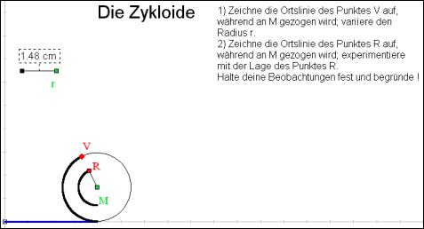
Beispiel für den TI 92
|
|
|
|
Hier ist die Zuggerade, der Startpunkt A der Zykloide und der Zugpunkt mit einer zur Geraden senkrechten gezeichnet. |
Hinzu gekommen ist der Hilfskreis um den Zugpunkt. Zugpunkt und der Rollkreis mit gleichem Radius. Der Abstand des Punktes A zum Zugpunkt wird auf den Rollkreis übertragen., der Punkt R. |
|
|
|
|
Die Hilfskonstruktionen sind ausgeblendet. |
Die Ortskurve des Punktes R , entstanden durch Ziehen des Zugpunktes. |
|
Fig. 12 a-d |
|
Beispiel:
|
Bei Zahnschaltgetrieben – Gangschaltungen – kommt das Planetengetriebe oftmals zur Anwendung, da es den Vorteil einer großen Leistungsdichte, geringer Geräuschentwicklung und Gleichachsigkeit von An- und Abtrieb hat. Hierbei ist entweder das Sonnenrad oder das Hohlrad festgesetzt. Die Abrollbahn ist in diesem Fall ein Kreis (s. Fig. 13). Klassifizieren Sie die Graphen der Ortskurven eines Punktes P. |
|
|
Fig. 13: Das vereinfachte Prinzip eines Planetengetriebes |
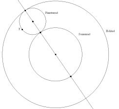
Lösungsskizze: Zwei Ansätze sind zu unterscheiden:
|
|
|
|
Fig. 14a: K1 rollt außen um K0 |
Fig. 14b: K1 rollt innen um K0 |


Die gepunkteten Linien sind die Kreise, auf denen sich die Mittelpunkte M1 bewegen.
Epizykloide – außen abrollender Kreis
Durch Einsetzen ergibt sich die endgültige Beziehung für außen abrollende Kreise in Abhängigkeit vom Drehwinkel und den Parametern r1 und r0
|
|
|
|
Für diesen Fall gibt es Möglichkeiten der Klassifikation
bei
festem Verhältnis der Radien zueinander und variabler Lage des Punktes P
bei
festem Punkt P und variablem Verhältnis der Radien
|
|
|
|
r1 : r0 = 1:3 und h > r1 |
r1 : r0 = 1:3 und h < r1 |
|
|
|
|
r1 : r0 = 1:3 und h = r1 |
r1: r0 = 1:1 und h = r1 |
|
|
|
|
Fig. 15 a-e |
r1 : r0 =3:4 und h = r1 |

Innen abrollender Kreis
Für innen abrollende Kreise gibt es die zwei Möglichkeiten, dass der Radius des rollenden Kreises K1 größer oder kleiner als der des Kreises Ko ist.
Die Beziehungen lassen sich für diese beiden Fälle in ähnlicher Weise erarbeiten wie im Fall des außen abrollenden Kreises. Als Ergebnisse erhält man die beiden folgenden Gleichungen:
|
|
|
|
|
Für die Hypozykloide gibt es ebenfalls die entsprechenden Möglichkeiten der Klassifikation.
Auch hier sollen an einigen Beispielen die Ortskurven vorgestellt werden.
|
|
|
|
r1 : r0 = 1:3 und h = r1 |
r1 : r0 = 1:3 und h > r1 |
|
|
|
|
r1 : r0 = 3:4 und h < r1 |
r1 : r0 = 3:4 und h = r1 |
|
Fig. 16a-d |
|

Ähnlich wie bei der Zykloide lassen sich Arbeitsblätter für die Beispiele der Epi- und Hypozykloiden herstellen, um die Abhängigkeiten graphisch sehr eindrucksvoll mit dynamischer Geometriesoftware experimentell zu erschließen und entsprechend motiviert anschließend algebraisch nachzuweisen.
5 Spiegelkabinett
Eine Parabel kann im x-y-Koordinatensystem leicht an allen Geraden gespiegelt werden. Verlaufen die Spiegelachsen parallel zur x- bzw. y-Achse, lassen sich auch die Terme der Bildkurven leicht ermitteln. Etwas schwieriger ist es schon bei der Spiegelung an der Winkelhalbierenden des 1. und 3. Quadranten.
|
Ermitteln Sie ein rechnerisches Verfahren zur Spiegelung der Normalparabel an der Geraden zur Funktionsgleichung y = 2x - 3. |
|
|
|
Fig. 17: Graphische Lösung |

Mögliche neue Fragen:
Lassen
sich auf ähnliche Art und Weise beliebige Kurven an
beliebigen Geraden spiegeln ? (Verallgemeinerung)
Welche
Kurve ergibt sich, wenn man nun die x-Achse an der Normalparabel spiegelt ?
(Umgekehrte Fragestellung)
Welche
Kurven ergeben sich, wenn man andere Geraden an der Normalparabel spiegelt ?
Diskussion
noch weitergehender Verallgemeinerungen.
Literaturhinweise
Fladt K. (1962) Analytische Geometrie spezieller Kurven. Akademische Verlagsges., Fankfurt.
Gray A. (1994) Differentialgeometrie. Spektrum Akademischer Verlag, Heidelberg.
Kreul and Kreul (1989) Funktionen und Kurven Bd. 2. Verlag Harri Deutsch, Leipzig.
Kreyszig E. (1957) Differentialgeometrie. Akad. Verlagsgesellschaft Geest & Portig, Leipzig.
Kroll and Vaupel (1986) Analysis für den Leistungskurs Bd. 2. Dümmler, Bonn.
Kühnel W. (1999) Differentialgeometrie. Vieweg, Braunschweig/Wiesbaden.
Lehmann E. (1990) Lineare Algebra mit Vektoren und Matrizen. Metzler Verlag.
Meyer J. (1996) Kegelschnitte mit Geometrie – Software.Mathematik betrifft uns Nr.5.
Meyer J. (1998) Von der Normalparabel zu kubischen Kurven. Beiträge zum Mathematikunterricht. Franzbecker, Hildesheim.
Steinberg G. (1998) Evoluten und Evolventen. MU Heft 4-5.
Steinberg G. and Ebenhöh, M. (1998) Ausgewählte Aufgaben zur Analysis. Schroedel, Hannover.
Strubecker, K. (1964) Differentialgeometrie I / II / III. Sammlung Göschen, Berlin.
Wieleitner H. (1908) Spezielle ebene Kurven. Göschen Verlagsbuchhandlung, Leipzig.
Wünsch, V. (1997) Differentialgeometrie. Teubner Verlag, Stuttgart.
Advantages and dangers
in the teaching of stochastics by using CAS
Otto Wurnig
Graz, Österreich
2. With CAS students can manage and understand algebraic proofs
3. Limit of sequences, summations and integrations of functions
4. The TI-92 can calculate in the graphic window
5. The TI-92 is a calculator with a spread sheet
6. The students can generate simulations with CAS calculators
1 Introduction
After the last reforms of the curricula in mathematics, statistics and the use of the computer were fixed in mathematical instruction for ten to fourteen year-old students (1993, 2000). With the use of helpful software it is now possible to give a first impression of such difficult concepts as linear regression and correlation to the students of grade 8. In the Austrian CAS II project in 1997/98, the use of the TI-92 was tested in many classes. The following four TI-92 pictures were made by the students grade 8 with their own dates (length and mass) to get a better understanding about the concepts of linear regression and correlation.
|
|
|
|
Fig. 1: Boxplot to the length |
Fig. 2: Histogram to the mass |
|
|
|
|
Fig. 3: Reg-line and corr-coeff |
Fig. 4: Points with the regression line |
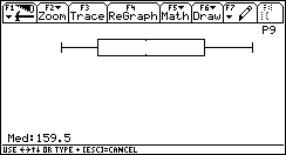
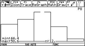
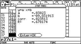

The possibility, to bring the TI-92 in action in many different mathematical situations, is certainly one of the important reasons, why the students of grades 7 and 8 like the TI-92 very much. The centre of school development (Zentrum für Schul-Entwicklung, ZSE) in Graz, an institute of the ministry of education, questioned the students in the Austrian CAS projects I and II. The result was that the fun in mathematics lessons increases with the use of the TI‑92 at every level, with PC-DERIVE this effect only turns up from grade 9 (15 year-old students) onwards (Grogger, 1995, 1999).
Probability & statistics are compulsory in the last grades of all schools, which are preparing students for university level. Unfortunately probability & statistics and the use of the computer became compulsory for teacher students at university only in the last few years. This is the reason why a young mathematics teacher still might not have a satisfactory knowledge of it. In order to improve this situation two organisations of mathematics teachers, the AMMU (Arbeitsgruppe für Modernen Mathematikunterricht) and the ACDCA (Austrian Center for the Didactics of Computer Algebra) have been founded.
The goal of the working group AMMU is to consider, how and to which extent the computer should be integrated in mathematical education, especially of business academies and secondary technical and trade schools, and in addition how it could help mathematics teachers to get new ideas and useful materials (homepage http://www.ammu.at/).
ACDCA organises conferences and meetings and makes publications with the intention to offer a framework for university teachers, teacher trainers and school teachers, especially of arts grammar and science grammar schools, to exchange their experiences and to do research projects (Homepage: http://www.acdca.ac.at/)
The following experiences were made in the last CAS III project of ACDCA (1999/2000). All students of the research class used TI-Derive or PC-Derive in the mathematics lessons and at home. The use of a CAS calculator is a very great advantage and gives new possibilities for solving problems especially in probability & statistics.
2 With CAS students can manage and understand algebraic proofs
With CAS calculators students can manage and understand algebraic proofs e.g. the derivation of the formula of the expectation and the variance of a binomial distribution, in the algebra window more easily and more independently.
|
|
|
|
Fig. 5: E(X): Calculation for n=20 u. n=50 |
Fig. 6: V(X): Calculation with two ways |
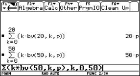
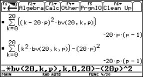
3 Limit of sequences, summations and integrations of functions
With CAS calculators students can manage and understand difficult concepts like limit of sequences, summations and integrations of functions in the algebra window
Problems of probability can thus quickly be solved without tables. The number of different ways of solving problems increases and stochastics loses its isolated position. Probability becomes a part of calculus.
The death rate of newborns, this means the probability of babies to die during their first year of life, is 1,8% in a country. What is the probability that of 1000 newborns chosen at random, more than 950 and less than 980 will live to see their first birthday? (Reichel 1992)
The probability that of 1000 newborn babies less than 21 will not live to see the first birthday is 73,1%; the contrary probability is 26,9%.
|
|
|
|
Fig. 7: BV: n = 1000, p = 0.982 |
Fig. 8: PV: l = n . p = 1000 . 0,018 = 18 |
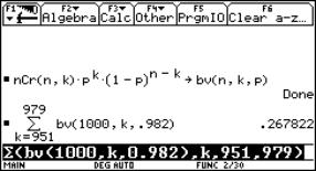
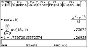
The binomial distribution can also be approximated by the normal distribution. With Derive this can be achieved by integration.
|
|
|
|
Fig. 9: NV(x,0,1) results in 27,6% |
Fig. 10: NV(x,µ,σ) results in 27,6% |
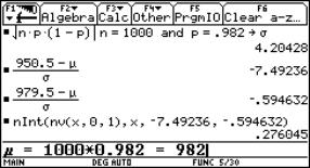
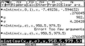
4 The TI-92 can calculate in the graphic window
The TI-92 can plot the Gaussian bell-shaped curve of the normal distribution in the graphic window for every µ and σ. If the curve is plotted, the TI-92 is able, with the command ∫ f(x).dx, to calculate the area under the curve after the input of the lower and upper bound
|
|
|
|
Fig. 11:Input of standardized corrected bounds |
Fig. 12: Input of corrected bounds 950,5;979,5 |
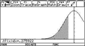
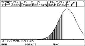
5 The TI-92 is a calculator with a spread sheet
If a table for the binomial distribution e.g. for n=20 and p=0,5; k = 0,1,2, ..., 20; is created in the data editor, a point diagram, a histogram and at last a probability density polygon is quickly plotted.
|
|
|
|
Fig. 13: Point diagram (square) |
Fig. 14: Width of the bars = 1 |
|
|
|
|
Fig. 15: Points as midpoints of the bars |
Fig. 16: Points connected (xy-line) |
|
|
|
|
Fig. 17: Probability polygon |
Fig. 18: The graph of nv(x,µ,σ) fits |
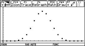
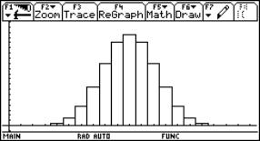
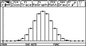
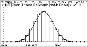
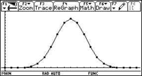
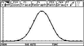
With this sequence of figures it is possible to get an imaginable transition from the discrete distribution to the continuous distribution including the important correction.
In order to replace the polygon with the fit curve of the probability density function nv(x,µ,σ), it is necessary to look for the standardized function with µ=0 und σ=1. If there is time, it is possible to go the way of standardization with all students stepwise (Wurnig, 1994, 2001), if there is no time, the function nv(x,0,1) can be entered and, on their own screens, all students can see that the curve is running through almost all the points.
How to get the function nv(µ,σ) ? → Standardization
|
|
|
|
Fig. 19a: Translation with (x-µ) |
Fig. 19b:Transformation: x→(x-µ)/ σ, y→σ.y |
|
|
|
|
Fig. 19c: Standardized points: n=20,25,30; p=½ |
Fig. 19d: The graph of nv(x,0,1) fits ! |
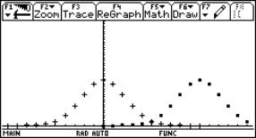
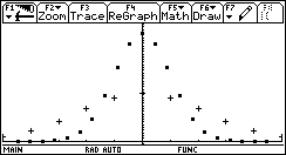
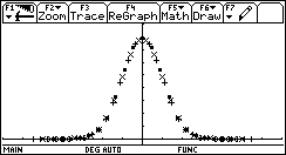
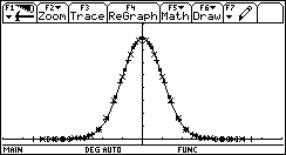
6 The students can generate simulations with CAS calculators
After entering CAS commands of their own, students can generate simulations with the random generator. Starting with real experiments they can find the right mathematical model with the help of simulations. A Laplacean die can be simulated by the TI die.
|
|
|
|
Fig. 20: 960 throws with the TI die |
Fig. 21: The TI die throws dice „well“ |
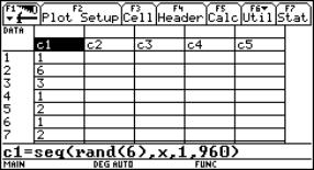
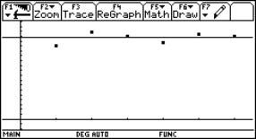
With the TI die the student is able to simulate the throw of coins without any further problems. In the following example 512 throws of a coin are simulated in row c1, c2, c3, c4. In the rows c5, c6, c7 the sums c1+c2, c1+c2+c3, c1+c2+c3+c4 are calculated. In this way it can be established, if the number or the heraldic figure of the coin turns up 0, 1, 2, 3, 4 times, when throwing two, three, four coins.
In order to save the trouble of counting the frequencies, the histogram can be made with the TI-92 and the absolute frequencies can be read in the graphic window with the trace mode.
|
|
throw with always one coin; c1, c2, c3, c4 c5=c1+c2 c6=c1+c2+c3 c7=c1+c2+c3+c4 |
|
Fig. 22a |
Fig. 22b |
|
|
|
|
Fig. 22c: Histogram for n=2, k=0, 1, 2 |
Fig. 22d: Histogram for n=3, k=0, 1, 2, 3 |
|
|
|
|
Fig. 22e: Input window to get a histogram |
Fig. 22f: Histogram für n=4, k=0, 1, 2, 3, 4 |
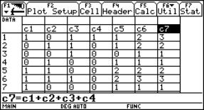
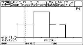
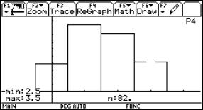
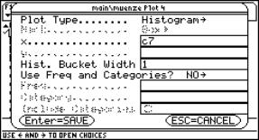
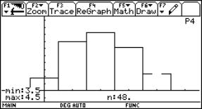
7 Concluding remarks
On the basis of the accompanying research of the CAS II project with the centre of school development (ZSE) it results that students who are mainly good at maths make positive observations and see advantages in the use of the TI-92 more frequently than those students who have good marks in their certificate in other subjects as well.
Furthermore the report points out that boys experience a stronger increase of fun than girls and a better stimulation of their interests and suffer less stress with the use of the TI‑92. Besides boys hardly notice a loss of mathematical basis knowledge (Grogger, 1999). All these reasons require a careful moving on when using utilities or functions and programs defined by the teacher. There is a great danger that such functions and programs are quickly used as a blind tool by the students. Thus, in this lecture, the function nv(x,µ,s) was used as the probability density function of the normal distribution without a further explication.
|
|
|
|
There is a danger, that the continuous use of self made function names makes students forget the official names and their mathematical meaning.
References
Grogger, G. (1995) Der Einsatz von Derive im Mathematikunterricht an AHS. Ergebnisse einer bundesweiten Schülerbefragung 1993/94. Zentrum f. Schulentwicklung, ZSE-Report 6. Graz.
Grogger, G. (1999) Evaluation zur Erprobung des TI-92 im Mathematikunterricht an AHS. ZSE-Report 40. Graz.
Reichel, H.C., Müller, R., and Hanisch, G. (1992) Lehrbuch der Mathematik 8. Hölder-Pichler-Tempsky, Wien.
Wurnig, O. (1995) Meine Erfahrungen mit dem Computer im Mathematikunterricht bis zum integrierten Einsatz in Klasse 12. Reichel, H.-C. (ed.): Computereinsatz im Mathematikunterricht. B.I., Mannheim.
Wurnig, O. (2001) Wahrscheinlichkeitsrechnung und Statistik. Rechenschaftsbericht zum Projekt CAS III, 1999/2000. ACDCA..
[1] According to Mahoney (1994), Pierre de Fermat was born on August 17th 1601.
[2] I have attempted–simply out of curiosity– to determine the origin of the use of the ‘little.’ One doesn’t find it in many standard, fairly recent classics (Hardy and Wright, Davenport, etc), whereas it is used in others, too numerous to mention. A query to the Number Theory Mailing List at nmbrthry@listserv.nodak.edu has elicited a great variety of suggestions, and I hope by the time of my Klagenfurt talk to have a clearer picture.
[3] Since no one has undertaken to write a book called Fermat’s little theorem. A thorough fleshing out of the wide range of topics I intend covering in my talk would indeed fill a substantial book.
[4] The names of some functions and some text in screen shots may seem strange to an English speaking reader. This comes because this paper and all programs were originally written in German. But from the context this difficulty will easily be overcome.
[5] The author isn’t quite sure whether this is the correct English expression. Another name might be coordinate form.
[6] Kavalierprojektion, Militärprojektion and Isometrie are German terms for that kinds of projection. The author doesn´t know the English names.